Ethics and Professional Standards
1. Ethics and Trust in Investment Profession, 2. Code of Ethics & Standards of Professional Conduct
Basics:
Ethics: Set of moral principles / rules of conduct providing guidance for behavior
Moral / ethical principles: beliefs on good / acceptable / obligatory VS bad / unacceptable / forbidden
Ethical conduct: behavior following moral principle / balances self-interest w in/direct consequences on other
Code of Ethics: Established general guide on org’s value / overall expectation regarding member behavior
Standards of Conduct: Established minimally acceptable / benchmark behaviors required by group enhancing Code of Ethics
Profession (1) are subject to license / technical standard (2) aim to serve society, set / enforce professional conduct
Professions build trust as they (1) normalize practitioner behavior (2) provide service (3) are client focused [fiduciary duty acting in best interest for another party] (4) have high entry std (5) possess expert knowledge [knowhow & synergy] (6) encourage continuing education (7) monitor conduct (8) are collegial / respectful (9) recognize oversight bodies (10) encourage member engagement (11) evolve (12) are professional (13) trust investment mngmnt [full disclosure]
Client interest < market interest
CFA Institute Global Body of Investment Knowledge (GBIK) and Candidate Body of Knowledge (CBOK) are updated thru practice analysis (interaction w practicing investment mngmnt professionals) to maintain body of knowledge relevant
CFA charterholders and CFA Program candidates are required to adhere to Code and Standards and to sign annually a statement attesting to that continued adherence
Investors w low levels of trust are less willing to accept risk and will likely demand a higher return for use of their capital
Investment management profession and investment firms must be interdependent to maintain trust
Challenges:
Overconfidence: too much emphasis on internal trait / intrinsic motivation
situational influence: money, prestige, loyalty
Legal vs ethical: Ex. trading w material nonpublic info - ok legally, unethical in CFA
Ethical Decision-Making Framework
Identify: Relevant facts (fact / opinion / bias) stakeholders and duties owed, ethical principles, conflicts of interest
Consider: Situational influences, additional guidance, alternative actions
Decide and act
Reflect: Was the outcome as anticipated? Why or why not?
Guidance:
Standards of Practice Handbook (Handbook) guides ethical dilemmas which all members must adhere to
CFA Institute Bylaws and Rules of Procedure for Professional Conduct (Rules of Procedure) structure the Code and Standards
CFA Institute Board of Governors oversee Professional Conduct Program (PCP). PCP and Disciplinary Review Committee (DRC) enforces Code and Standards. DRC reviews conduct and partners with Professional Conduct (PC) staff to establish / review professional conduct policies. PC division enforces test policies and professional conduct of Certificate in Investment Performance Measurement (CIPM). CFA Institute Standards of Practice Council evaluates Code and Standards and Handbook, ensuring they are effective (representative of high standards, relevant, applicable, comprehensive, enforceable, testable)
PC inquiries:
Source: (1) self disclosure on annual PC Statement - litigation, investigation (2) written complaint received by PC staff (3) media, regulatory notice, public source (4) proctors monitoring test (5) score analysis to detect disclosure of confidential exam info
Conduct interviews / investigation
Result: no disciplinary action, issue cautionary letter, continue proceedings to discipline member
Rejection or acceptance by members. If rejected, matter referred to DRC
Sanctions include public censure, suspension of member / use of CFA design, revocation of CFA
Code of Ethics:
Act w integrity, competence, diligence, respect and ethically w public, clients, prospective clients, employers, employees, colleagues in investment profession, other participants in global capital markets
Place integrity of investment profession, interests of clients above own personal interests
Use reasonable care, exercise independent professional judgment when conducting investment analysis, making investment recommendations, taking investment actions, engaging in other professional activities
Practice, encourage others to practice professional, ethical manner reflecting credit on themselves, profession
Promote integrity, viability of global capital markets for the ultimate benefit of society
Maintain, improve professional competence, strive to maintain, improve competence of other investment professionals
Standards of Professional Conduct: (Revisions of 11th version underlined) in Standards of Practice Handbook
Professionalism
Knowledge of the Law
Members must understand / comply w all applicable laws, rules, regulations (Code & Standard) of any gov, regulatory organization, licensing agency, professional association governing their professional activities. In event of conflict, Members must comply with the more strict law, rule, regulation. Members must not knowingly participate / assist in and must dissociate from any violation of such laws, rules, or regulations.
→ (1) attempt to stop behavior by bringing it to attention of employer thru supervisor / compliance department. (2) members dissociate from activity (removing own name in written reports, asking for dif assignment, refusing to accept new client / continue current)
→ if using photocopy of paid textbook, both user and provider are in violation
Independence and Objectivity (VS VI (A) Disclosure of Conflict)
Members must use reasonable care, judgment to achieve, maintain independence and objectivity in professional activities. Members must not offer, solicit, accept any gift, benefit, compensation, consideration that reasonably could be expected to compromise their own or another’s independence and objectivity.
→ allocation of shares in oversubscribed IPOs to investment managers for their personal accounts is prohibited
→ If possible, disclose gifts before accepting, and if impossible, disclose to employer benefits
→ To miniminze pressure from IB, use (1) enhanced firewall: separate reporting structures for personnel on research & IB side (2) good compensation for research analysts (3) comp’s regular policy review to safeguard analysts
→ If pressure by comp to change rating, place comp on restricted list, give facts only ab comp
Misrepresentation
Members must not knowingly make any misrepresentations relating to investment analysis, recommendations, actions, other professional activities.
Misconduct
Members must not engage in any professional conduct involving dishonesty, fraud, deceit or commit any act that reflects adversely on professional reputation, integrity, competence.
Integrity of Capital Markets
Material Nonpublic Information
Members who possess material nonpublic info that could affect the value of investment must not act or cause others to act on the info
→ Mosaic theory: use non/material non/public info to create larger picture, and conclusion becomes material after assembled
→ Build firewall to keep material nonpublic info
→ If hear material nonpublic info on security, place it on restricted list - you can not act on it even if personal account
Market Manipulation
Members must not engage in practices that distort prices, artificially inflate trading volume w intent to mislead market participants.
Duties to Clients:
Loyalty, Prudence, and Care
Members have a duty of loyalty to their clients, must act with reasonable care and exercise prudent judgment. Members must act for the benefit of their clients, place their clients’ interests before their employer’s or their own interests.
→ soft commission policy: members are required to only use client brokerage to the benefit of the clients
Fair Dealing
Members must deal fairly, objectively w all clients when providing investment analysis, making investment recommendations, taking investment action, engaging in other professional activities.
Suitability
When Members are in an advisory relationship with a client, they must:
Make a reasonable inquiry into a client’s or prospective client’s investment experience, risk and return objectives, financial constraints prior to making any investment recommendation, taking investment action and must reassess, update this info regularly.
Determine that an investment is suitable to the client’s financial situation and consistent with the client’s written objectives, mandates, constraints before making an investment recommendation or taking investment action.
Judge the suitability of investments in the context of the client’s total portfolio.
When Members are responsible for managing a portfolio to specific mandate, strategy, style, they must make only investment recommendations or take only investment actions that are consistent with the stated objectives and constraints of the portfolio.
Performance Presentation
When communicating investment performance info, Members must make reasonable efforts to ensure it is fair, accurate, complete.
→ Standards do not require compliance with GIPS, auditing, verification requirements
Preservation of Confidentiality
Members must keep info about current, former, prospective clients confidential unless:
Info concerns illegal activities of prospective / client,
Disclosure is required by law,
Prospective / client permits disclosure of the info.
→ in case illegal activity detected: seek guidance from employer → legal counsel → resign
Duties to Employers
Loyalty
In matters related to their employment, Members must act for the benefit of their employer and not deprive their employer of the advantage of their skills and abilities, divulge confidential info, or otherwise cause harm to their employer.
→ In case member enters into independent biz while still employed, members must notify and earn consent of employer, describe type of service rendered, expected education of service, compensation for the services
→ soliciting clients is strictly prohibited when leaving a comp unless the solicited is unemployed
Additional Compensation Arrangements
Members must not accept gifts, benefits, compensation, consideration that competes with or might reasonably be expected to create a conflict of interest with their employer’s interest unless they obtain written consent from all parties involved.
Responsibilities of Supervisors
Members must make reasonable efforts to ensure that anyone subject to their supervision or authority complies w applicable laws, rules, regulations, Code and Standards.
→ if member cannot fulfill supervisory responsibilities due to absence of compliance system, member should decline in writing to accept supervisory responsibility until firm adopts reasonable procedures to allow member to exercise responsibility
Investment Analysis, Recommendation, and Actions
Diligence and Reasonable Basis
Members and Candidates must:
Exercise diligence, independence, thoroughness in analyzing investments, making investment recommendations, taking investment actions.
Have a reasonable, adequate basis, supported by appropriate research, investigation, for any investment analysis, recommendation, action.
→ Selecting External Sub/advisor: (1) reviewing adviser’s established code of ethics, (2) understanding adviser’s compliance, internal control procedures, (3) assessing qual of published return information, (4) reviewing the adviser’s investment process and adherence to its stated strategy.
Communication with Clients and Prospective Clients
Members and Candidates must:
Disclose to prospective / clients the basic format and general principles of investment processes they use to analyze investments, select securities, construct portfolios and must promptly disclose any changes that might materially affect those processes.
Disclose to prospective / clients significant limitations, risks associated w investment process.
Use reasonable judgment in identifying which factors are important to their investment analyses, recommendations, actions and include those factors in communications with prospective / clients.
Distinguish between fact, opinion in presentation of investment analysis, recommendations.
Record Retention
Members must develop, maintain appropriate records to support their investment analyses, recommendations, actions, other investment-related communications with prospective / clients.
Conflicts of Interest
Disclosure of Conflicts
Members must make full and fair disclosure of all matters that could impair their independence and objectivity or interfere with respective duties to their prospective / clients, employer. Members must ensure that such disclosures are prominent, are delivered in plain language, communicate the relevant info effectively.
→ If my senior is a board of subsidiaries of comp I write a research on, I disclose the relationship
→ If I write a research about comp A, and my comp holds stock of A, I need to disclose. No need to disclose I purchsed A stocks, or my brother is a supplier to A
Priority of Transactions
Investment transactions for clients and employers must have priority over investment transactions in which a Member is the beneficial owner.
Referral Fees
Members must disclose to their employer, prospective / clients, as appropriate, any compensation, consideration, benefit received from or paid to others for the recommendation of products or services.
→ disclosure allows client / employer to evaluate (1) any partiality shown in any recommendation of service (2) full cost of service.
Responsibilities as a CFA Institute Member / Candidate
Conduct as Participants in CFA Institute Programs
Members must not engage in any conduct that compromises the reputation or integrity of CFA Institute or the CFA designation or the integrity, validity, security of CFA Institute programs.
Reference to CFA Institute, the CFA Designation, and the CFA Program
When referring to CFA Institute, CFA Institute membership, the CFA designation, or candidacy in the CFA Program, Members must not misrepresent or exaggerate the meaning or implications of membership in CFA Institute, holding the CFA designation, or candidacy in the CFA Program.
→ O: I enrolled in the CFA Program to obtain the highest set of credentials in the global investment management industry.” “I Passed level 3 CFA exam”
→ “Chrissy is a CFA,” partial designation, “I got the highest score in the test”
** Party / nonmember / fim can claim compliance w CFA Institute Code & Standard once they have ensured that their code and ethics meets the principles of the Code and Standards.
4. Global Investment Performance Standards (GIPS)
Mission: promote ethics and integrity and instill trust through the use of the GIPS standards by achieving universal demand for compliance by asset owners, adoption by asset managers, support from regulators for the ultimate benefit of the global investment community.
Objective:
Promote investor interests, instill investor confidence.
Ensure accurate, consistent data.
Obtain worldwide acceptance of a single standard for calculating, presenting performance.
Promote fair, global competition among investment firms.
Promote industry self-regulation on a global basis.
Any firm that manages actual asset may comply. Firm must create, maintain composites for all strategies which firm manages segregated accounts. Firm must include all actual fee-paying, discretionary segregated accounts in at least one composite defined by (the same) investment mandate, objective, or strategy. Pooled funds must also be included in any composite for which the pooled fund meets the composite definition. This prevents cherry-picking
→ no non-discretionary segregated account, non-feepaying account
Verification: must be performed firm-wide. Compliance is claimed by comp, but verification by 3rd party
Composition (FICCDPRPW)
Fundamentals of compliance: Use “in accordance,” “in compliance,” “consistent.” Provide a compliant description of the past 12 months to all prospective clients. The firm may select its sub-advisor, but all total firm assets must be assigned to the sub-advisor
Input data
Calculation methodology
Composite construction
Disclosure: Performance / policies adopted by firm
Presentation and reporting
Real estate: not including publicly traded real estate securities, CMBS, private debt investment, frequency of external valuation
Private equity
Wrap Fee / Separately Managed Account (SMA) portfolios
** 6~9 are not under required provisions
The minimum effective compliance date for a wrap fee composite is 1 January 2006
• 1 January 2006 for real estate and private equity composites and pooled funds, as well as wrap fee composites.
• 1 January 2000 for all other composites and pooled funds.
Firm must maintain a list of composite descriptions and include terminated composites on this list for at least 5 years after the composite termination date. A complete list of pooled fund descriptions for limited distribution pooled funds is also required. A complete list of broad distribution pooled fund names only, but not the descriptions, is required. Firms are not required to include terminated limited or broad distribution pooled funds on the list.
Requirements:
The firm must present GIPS compliant record of a min 5 yrs of annual investment performance. If existent for less than 5, must present performance since inception. Afterwards, present additional year performance for each year to min 10 yrs
Firms may internally self-regulate, but should hire a 3rd party to perform legitimate composite testing and have local sponsoring org for effective investment performance standards.
Must comply to consistent data import and have blackout period (3 days employees not allowed to make alterations to a big retirement / investment plan), pre-clearance (obtain clearance – approval – before making the trade)
Recommend to input office locations, not overcrowd participation in IPO
Quantitative Methods
1. Rates and Returns
2. Time Value of Money
ROR = YTM = I/Y, discount rate = int rate, coupon = PMT
Annuity [finite, level CF / PMT]:
Ordinary annuity: CF indexed at t = 1 (end of payment period, usual format)
Annuity due: CF indexed at t = 0
Continuous compounding: FV = PV erN with N standard 1 year
Perpetual bond [infinite]: PV = PMT/(rs/m)
Constant dividend: PVt = Dt/r
Constant / Gordon Growth DDM Model : [Same as Cost of Equity’s V0]
PVt = Dt(1+g)r-g = D1r-g
Assumptions: (1) Div is correct metric for valuation (2) Div growth / Required ROR forever (3) Div growth rate < Required ROR
For insensitive to biz cycle, mature growth phase
Ex. electric utility serving a slowly growing area or a producer of a staple food product
* Cost of Equity V0 = D0(1+g)r-g = D1r-g
* WACC: re = D1P0 (1-f) + g
Multi-stage growth model:
PVt =(1) i=1nDt (1+gs)i(1+r)i + (2,3) E(St+n)(1+r)n where E(St+n) = Dt+n+1 (r-gl)
(1) ST Div Cost: find ∑(individual ST Div cost)
(2) LT Div Cost: find E(St+n) = terminal value = stock value of the stock in n periods: [Dt+1 (1 + LT growth)] / (r-gl)
(3) (2) / (1+r)n
(4) add (1) and (3)
For rapidly growing companies
* Cost of Equity V0 = t=1nD0(1+gs)t(1+r)t + Vn(1+r)n , where Vn Dn+1r-gL , Dn+1 = D0 (1+gs)(1+gL)
Price to Earning ratio
Price to Earning ratio = pr-g, p = Div Payout Rate
As PVt = Dt (1+g)r-g=> PVtEt = Dt (1+g) / Etr-g
Forward price to earning ratio: = Expected div payout ratior-g
As PVtEt+1 = Dt+1 (1+g) / Et+1r-g
Different CF: Find NPV, and compare to other investment’s PV
Two Rf bonds: F1,1 = (1+r2)2/(1+r1) -1
As FV2 = PV0(1+r2)2 = PV0(1+r1)(1+F1,1)
Options
V0 = (hedge ratio) S0 - c0 = Vu1+r = Vd1+r
Hedge ratio: Proportion of underlying offsetting risk associated with a deriv position = Units that investor is buying
Portfolio value = V
Vu, Vd= (hedge ratio)(up side of binomial) - (Up’s contract value) = (hedge ratio)(down side of binomial) - (Down’s contract value)
3. Statistical Measures of Asset Returns
Parameter: Descriptive measure of a population characteristic
Measures of Central Tendency:
Measures of Dispersion:
Measures of Shape Distribution:
Measures of Location: Quantile
Percentile: 10th percentile = 0~10% upper bound
Interquartile range (IQR) = Q3-Q1
Yth percentile (Py) using linear interpolation. Ex. 2nd quartile: y = 50%
Box and whisker plot’s middle point = median
Measure of relationship:
Correlation: measures linear relationship between two random variables, -1~1, 0 no relationship
Covariance: measures joint variability between two random variables
If cov positive, cor positive
| Measure of Loc | Population | Sample |
Central tendency | Observed | Parameter | Sample |
Mean | μ | X̄ |
Dispersion | Variance | σ2 , uses n | 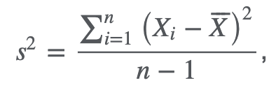
|
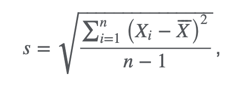
Standard deviation | σ, uses n
| 
|
Relationship | Correlation Corr(X,Y) | ρ = σXY / σXσY | r = sXY / sXsY |
Covariance Cov(X,Y) | σXY = ρσXσY | sXY = ρsXsY |
4. Probability Trees and Conditional Expectations
5. Portfolios Mathematics (Different weights)
Expected return of portfolio: E(RP) = w1E(R1)+w2E(R2)+…+wnE(Rn)
Variance: σ2(RP) = E [{RP-E(RP)}2] = i=1nj=1nwiwj Cov(Ri,Rj)
Total n variances
Ex. σ2(Rp) = w12σ12(R1) + w22σ2(R2) + 2w1w2 Cov(R1,R2)
Ex. σ2(Rp) = w12σ12(R1) + w22σ2(R2) + w32σ2(R3) + 2w1w2 Cov(R1,R2) + 2w1w3 Cov(R1,R3) + 2w2w2 Cov(R2,R3)
Covariance: Population Cov(Ri,Rj) = E [(Ri-ERi)(Rj-ERj)]
Total n(n − 1)/2 covariances
Shows how co-movements of returns affect aggregate portfolio variance, directions
-∞ ~ ∞
Cov(Ri,Rj) = ρ(Ri,Rj) [σ(Ri)σ(Rj)]
** Covariance with itself: used to find std dev by rooting
Correlation: ρ(Ri,Rj) = Cov(Ri,Rj)/[σ(Ri)σ(Rj)]
Joint probability function P(X,Y): Cov(RA,RB) = ij P(RA,i,RB,j) (RAi-ERA) (RBj-ERB)
In other words, find probability for both cases, subtract that from the percentages, multiply together, multiply w probability
Probability of joint occurrences of values of X and Y
ER = Expected return = Σ (Probability × RA)
R = Return
Ex.
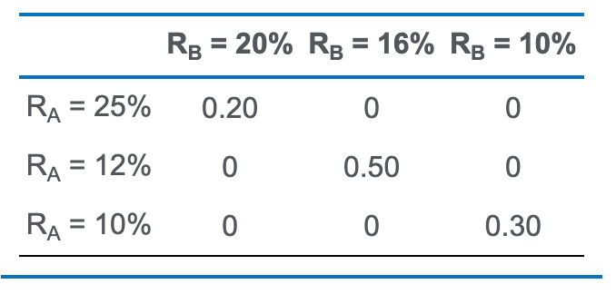

Independence: if P(X,Y) = P(X)P(Y)
* Stronger than uncorrelated
Uncorrelated: if E(XY) = E(X)E(Y)
Modern Portfolio Theory: Mean-variance analysis,
Safety-first ratio = [E(RP) - RL] / σP
higher SF 🙂
= Distance from TH / sd = units of deviation
Measures downside risk, RL = Threshold, assumes normal distribution
Stress testing, scenario analysis: set of techniques for estimating losses in extremely unfavorable combinations of events or scenarios
Value at risk (VaR): money measure of the min value of losses expected over a time period at a given level of probability
6. Simulation Methods
Lognormal Distribution
Continuously compounded return = Ln (End / Beg)
Skewed right, lower bound of 0
Parameter: mean, std of its normal distribution
Current stock’s continuously compounded return is normally distributed → future stock is lognormally distributed
Assumes: Independently and identically distributed (i.i.d.): Random variables that are independent of each other but follow the identical probability distribution
If not normally distributed, sum is normal due to central limit theorem
More suitable as probability model for asset price, not suitable for asset return (both pos & neg)
Monte Carlo simulation: Inverse transformation method to convert ‘randomly generated uniformly distributed number → ‘simulated value of random variable of desired distribution.’ However, it is an estimate that can not specify cause-and-effect relationship. For predicting modeling, quantifying risk
Resampling: Resampling from single sample for the statistical parameters / estimates like std error, confidence intervals, robustness
Bootstrap method: replace the observed
Jackknife method: no replace, sample size = n = repetition time
7. Estimation and Inference
Probability sampling (random):
Simple random sampling, systematic sampling (kth),
Stratified sampling: divide into strata / subpopulations / index, then simple random sampling from each strata
Cluster sampling: divide into clusters, clusters chosen by simple random sampling
Non-probability sampling: convenience sampling, judgemental sampling
Central limit theorem: larger sample around 30 allows
8. Hypothesis Testing, 9. Parametric and Non-Parametric Tests of Independence
Testing subject | Test statistic | DoF | Info |
| Z = (X-μ) / (σ-√n) |
| Known population variance, large / normal sample, σ 68, 2σ 95, 3σ 99% 90% confidence intervals: z0.05 = 1.65 2σ 95% confidence intervals: z0.025 = 1.96 3σ 99% confidence intervals: z0.005 = 2.58
n stocks, n means, n variances, (n(n-1)) / 2 correlations |
Single mean | t = X̄- μ0s/n | n-1 | Unknown sample or pop variance, large sample Not normal (2 random variables of sample mean, std dev), becomes normal as sample ↑ |
Dif btw means | 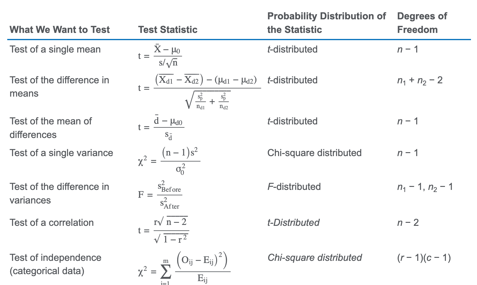
| n1 + n2 - 2 | 2 independent samples, 1 sided test H0: μ1- μ2 = 0, so rightside of top = 0 sp2 = (n1-1)s12+ (n2-1)s22n1 + n2 - 2 = pooled estimate of variance IF unequal and unknown pop variance. sp is replaced with s1 and s2 |
Mean of dif | t = đ- μd0sd / √n Paired comparison test | n-1 đ | 2 dependent samples approx normal dist, unknown but assumed equal variance sđ = sd / √n sd = standard deviation difference đ = mean difference = 1ni=1ndi H0: μd0 = 0, so rightside of top = 0 |
Single variance or std dev | 𝛘2 = (n-1)- s2σ02 | n-1 | 1 sided test (asymm), normal distribution σ02 = trigger level ↑n = pdf shape becomes bell curve |
Dif variance | F = s2Befores2After | n1 - 1, n2 - 1 |
|
Pearson / Bivariate Correlation | t = r n-21-r2 | n-2 | R = sample correlation |
Independence | 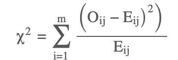
| (r-1)(c-1) | Categorical, discrete data using contingency / two-way table, 1 side rejection region H0: size and type are not related / are independent M: num of cells in table O: observed frequency E: expected number of observation assuming independence |
Result \ Reality | True H0 | False H0 |
Fail to reject H0 (Accept H0) | :) 1-α = Confidence level | False negative, Type 2 error = β |
Reject H0 | False positive = False Discovery Rate (FDR, worse), Type 1 error α = significance level | :) 1-β = Power of test |
Non-parametrics: For (1) data does not meet distributional assumptions, (2) there are outliers, (3) data is given in ranks / uses ordinal scale, (4) relevant hypotheses does not concern a parameter. Types include:
Single mean (z, t) → Wilcoxon signed-rank test
Dif btw means (t) → Mann-Whitney U test
Mean differences (t) → Wilcoxon signed-rank test, Sign test
Spearman rank correlation coefficient: rs
Rank observation large (1) to small (n), [if tied, av of joint ranks 3.5]
Calculate dif di between ranks for each pair for X, Y, and find di2
rs = 1 - 6 6i=1ndi2n(n2-1)
10. Simple Linear Regression (SLR)
SLR: method to estimate relation in/dependent variable. Requires minimizing of Sum of Squares Error (SSE, residual sum of squares)
Yi = b0 + b1Xi + εi, i = 1, . . . , n.
Variables:
Y: dependent variable, explained variable, [Calc: Needs to be inputted in second]
X: independent variable, explanatory variable
b0: intercept, regression coefficient, [Calc: as a]
b1: slope coefficient, regression coefficient [Calc: as b]
εi: error / residual = Yi - Ŷ. Least squares RL should have εi = 0
r: correlation = cov (Y,X) / SY SX
Cov(Y,X) = i=1n(Yi - Ȳ)(Xi-X̄)n-1 (X here is X̄), top: Sum of cross-products of deviations from the mean
SY = i=1n(Yi - Ȳ)2n-1
SX = i=1n(Xi - X̄)2n-1 (X here is X̄)
Sum of Squares Total (SST): Variation of Y
= i=1n(Yi - Ȳ)2 = SSE + SSR
Sum of Squares Regression (SSR): explained variation in Y
= ∑(Ŷi - Ȳ)2
= expected - mean
Sum of Squares Error (SSE): Unexplained variation / error / residual in Y
= i=1n(Yi - Ŷi)2 = i=1n[Yi - (b̂0 + b̂1 Xi)]2 = i=1nei2
= observed - expected
Assumption:
Linearity: Relationship between X & Y is linear
Homoskedasticity: Variance of regression residuals are same for all observations
Independence: Observed pairs of X and Y are independent, and regression residuals are uncorrelated across observations
Normality: normally distributed regression residual (not variable)
Measures of Goodness fit:
= SSR / SST
** If slope is positive, correlation (X,Y) = √R2
= se / √i=1n(Xi-X̄̄)2
= 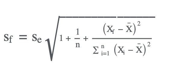
Prediction interval: Ŷf ± tcritical for 𝛂/2 sf
Log-lin model: LnYi = b0 + biXi
Lin-log model: Yi = b0 + b1lnXi
Log-log model: LnYi = b0 + b1lnXi
11. Introduction to Big Data Techniques
Fintech: technology-driven innovation occurring in the financial service industry
Big Data: collection of large quantities of financial data from a variety of sources in multiple formats
Expert system (computer if-then) → neural networks (brain) → machine learning (train / validate / test. Can seem like “black box” or opaque = not fully understandable outcome. Has downsides of overfitting [too cognizant], underfitting. Techniques include supervised learning [only data] / unsupervised learning [labeled] / deep learning [neural networks to find patterns])
Data science: interdisciplinary field harnessing advances in computer science (ML), statistics to extract info from big data. Processing methods include:
Capture: Data collection / formatting for analysis. Needs low latency systems for real time calculation
Curation: Ensure data quality thru cleaning.
Storage: Data record / archive / access
Search: Querying requested data
Transfer: Move storage location to analytical tool
Data visualization: tag cloud (text size = importance), text analytics (large unstructured text like company filings- for ST trends), Natural Language Processing (interpreting human language / translation)
Economics
1. Firm and Market Structures
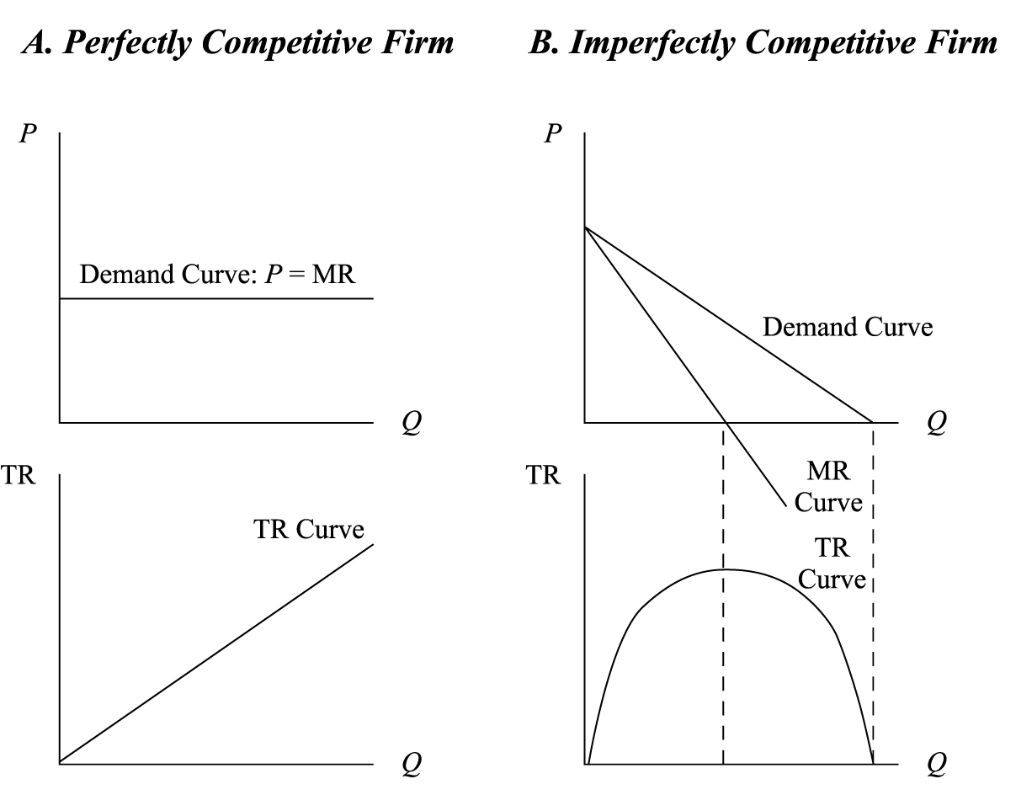
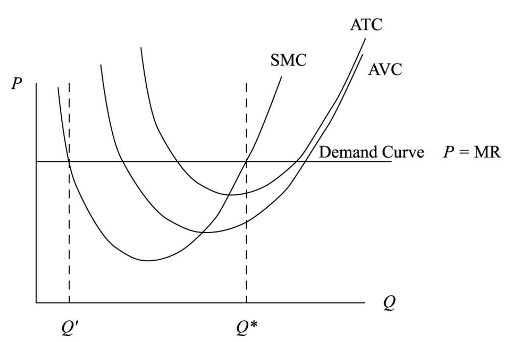
Perfectly competitive
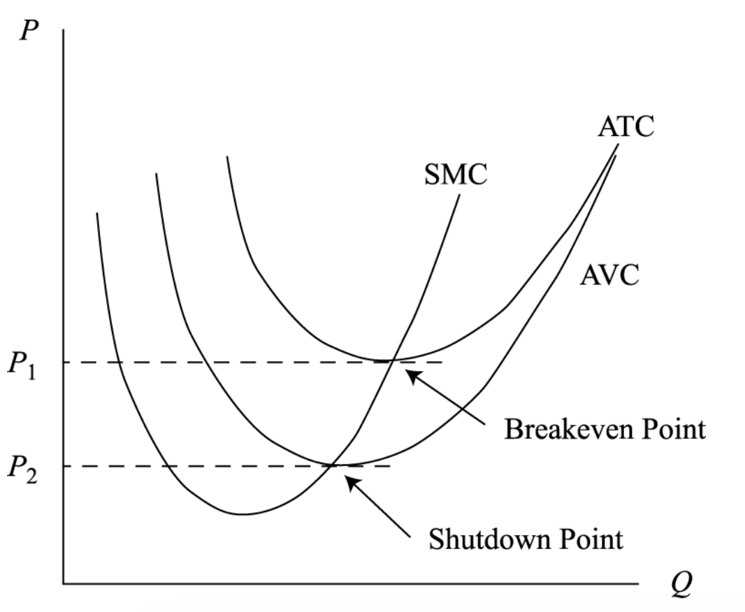
Perfectly elastic (horizontal) demand curve: P = MR
Supply = MC
Average Rev (AR) = price per unit
TR = (P)(Q)
Break even: P (= MR) = AR [TR = TC or AR = ATC]
Monopolistic Competition
Characteristic: competitive, unique product, lower barrier to entry, advertising helps profit
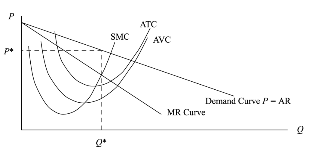
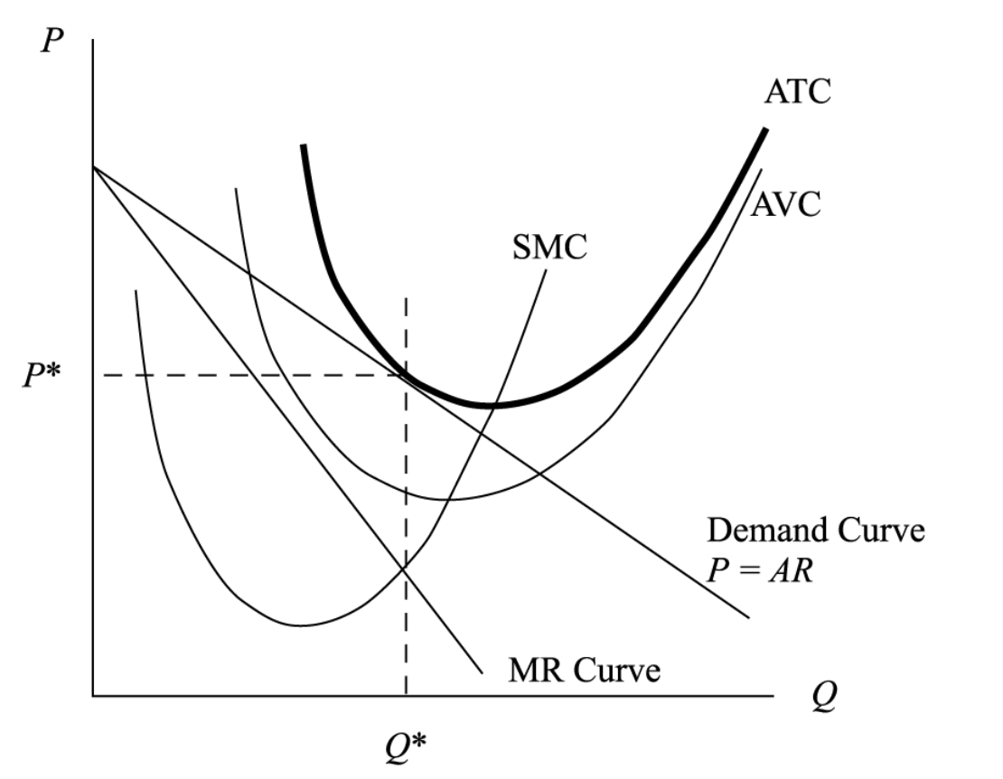
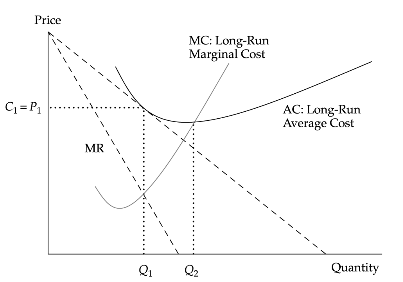
Profit Maximization: MR = MC
Negatively sloped demand curve: P = f(Q), P > MR, P = AR
No supply function
TR = f(Q) × Q
Break even: P (= AR) = ATC [TR = TC or AR = ATC] [3rd pic]

Oligopoly:
Characteristic: Few sellers, standard product, advertising a lot. Attracts collusion
Profit Maximization: MR = MC
No supply function
Pricing strategy:
Pricing interdependence:
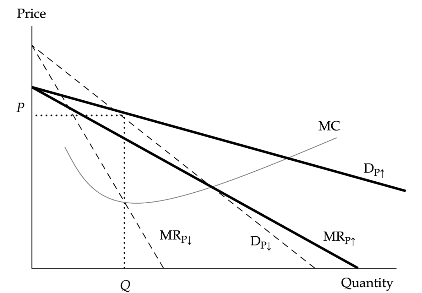
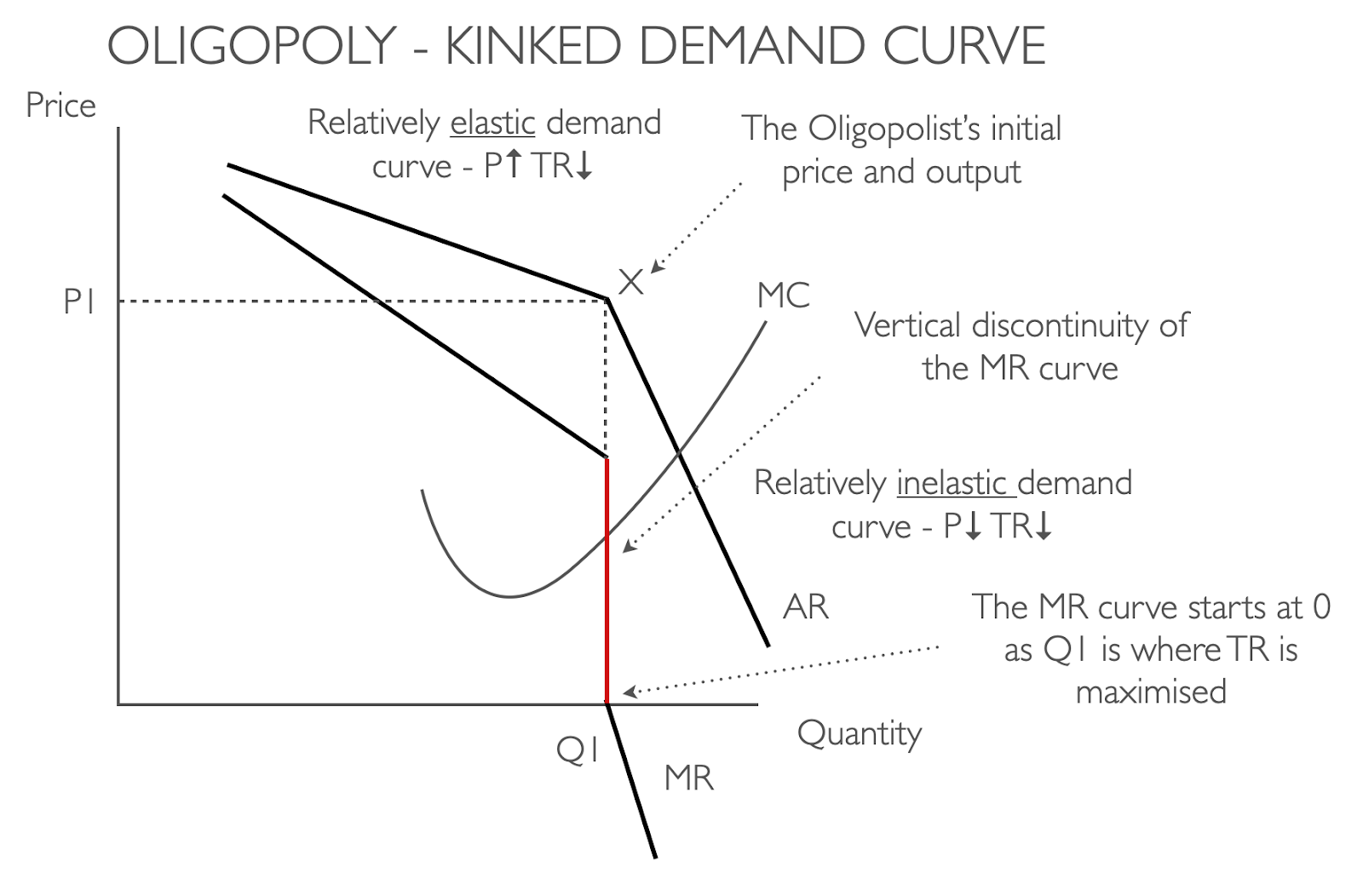
Competitors will lower prices to match a price reduction, but will not match a price increase
Can’t determine prevailing price, explains stable prices (red)
Cournot assumption: Firm determines profit maximizing production lvl assuming other firm does not change output. In LT equilibrium, output / price are stable, no increase profits either
Nash equilibrium: Collusion / cartel allows higher prices. collusion more likely if (1) small number of firms / one dominant firm, (2) homogenous product (3) similar cost structure (4) frequent and small order size (5) less likeliness for retaliation (6) high external competition
Stackelberg model: A prominent model of strategic decision making in which firms are assumed to make their decisions sequentially.
If dominant decreases price, smaller comp will leave market rather than sell below cost, thus market share of price leader (dominant comp) will increase. In LT, market share of dominant comp decreases as profits are shared by more participants
Monopoly:
Characteristic: One seller, unique product, advertising does not help profit
Profit Maximization: Max (TR-TC = π)
Others:
Constant returns to scale: same cost per unit (↑ X input = ↑ X Output)
Economics of scale: ↓ cost per unit
Market power: concentration ratio (0~100, ≠ market power, unaffected by merger), HHI (Σ Comp market share2, Use full number, not the percentage)
2. Understanding Business Cycles
Business cycles: recurrent expansions & contractions in economic activity (mostly GDP) affecting economy
Types:
Classical cycle: Level of economic activity measured by GDP volume terms. Contraction phase (between peaks / troughs) short, expansions large
Growth cycle: Economic activity by LT potential / trend growth level to see how actual economic activity does vs potential
Growth rate cycle: Growth rate of economic activity (GDP growth rate). Peaks and troughs recognized earlier
Phases:
Recovery (trough):
Below av: output worst (vs potential), economic activity (consumer / biz spending, start to increase), low int rate,
Above av: unemp rate
Decrease: negative output gap, layoff, decline in sale, inventory - sales ratio (sales increase faster than production)
Situation: moderate inflation, biz overtime (vs hire), capital spending (excess capacity / low utilization, CAPEX focus on efficiency / light product like software, systems, hardware - high rate of obsolescence)
When expansion is expected: Risky assets repriced upward, corps incorporate higher profit expectations into corp bond / stock prices
Expansion (boom):
Above av: growth rate, activity measures (but decelerating), sales production
Increase: Recovery, consumer spending, company, price / int rate, positive output gap, inflation, capacity utilization
Situation: Employment: overtime / temp → hiring, unemp stabilize / falls, capital spending (new orders focus on heavy / complex equipment, warehouse. factory), stable inventory-sales ratio, Shortage in factors of production, overinvestment in productive capacity may lead to reduce further investment spending
Late stage: biz experience a decrease in qualified workers, productive capacity limits ability to respond to demand
Slowdown (peak):
Above av: activity measures (decelerating), inflation (accelerate), output (vs potential output), consumer optimism, interest rate
Below av: rate of growth
Increase: inventory-sales ratio (weakening economy, sale slows)
Decrease: Growth rate (vs potential output growth), positive output gap, inflation, price level, hiring pace, factors of production (D>S), unemp rate (slower rate)
Situation: stable hiring (slower, rely on overtime), healthy CF, order cancellation
Contraction:
Below av: economic output (vs potential economic output), activity measures, growth
Increase: negative output gap
Decrease: demand, profit, CF, capital spending (CF, short lead time tech / equipment → heavy construction cut off), consumer / biz confidence, comp cost (overtime and hires), absolute economic activity (recession / depression), inflation (lag), employment (cut hours / eliminate overtime / freeze hire / layoff, unemp rate rise), inventory-sales ratio (falls to normal)
Situation: biz produce at rates below sales volumes necessary to dispose unwanted inventory
Economic Indicators
Leading: stock market (S&P), house price, retail sales, interest spread (10 Y treasury yield & overnight borrowing rate - federal fund. Bigger 🙂), building permits for new private housing units, consumer expectation, av weekly hours (manufacturing), manufacturer’s new orders for non-defense capital goods (excluding aircraft), av weekly initial claims to unemp insurance, ISM (Institute of Supply Management, indexes for manufacturing orders, output, emp. Bigger 🙂), LCI (Leading Credit Index, leading financial indicators showing strength of financial system)
Coincident indicators: industrial production index (industrial production reflects current state better than services), real personal income (on non-agri payroll), manufacturing / trade sales
Lagging: Av duration of unemp, inventory to sales ratio (good to maintain 10-20%, Smaller 🙂), change in unit labor cost, inflation (index includes stable service components), ratio of consumer installment debt to income (consumers borrow more when confident), commercial and industrial loans outstanding
Diffusion index: % of index’s components moving consistently w overall index. Reflects consensus change
Nowcasting: real-time monitoring of economic and financial variables to continuously assess current conditions and provide an estimate of the current state.
Credit cycle: Fluctuation of credit measured through liquidity of priv sector (loans, investment, real estate). Strong economy = loose credit (may contribute to asset price and real estate bubbles and subsequent crises)\
3-4. Policies
Policies: Stable / positive growth, stable / low inflation
Fiscal Policy: Influence on Taxation, Spending to control growth / GDP. Affects overall Aggregate Demand (AD) and activity, distribution of wealth / income, resource allocation
AD: amount companies and households plan to spend. Fiscal policy influences AD
Keynesians: Fiscal 🙂 on AD, output, esp if substantial spare capacity (considerate unemp) in economy
Monetarists: only temp effect on AD, monetary policy more effective to restrain / boost inflation
*Debt
Ok: debt may be owned by citizens or used for capital investment, private sector may offset fiscal deficits by increasing savings foreseeing increased taxes (Ricardian equivalence - reason to choose Monetary policy, future impact of fiscal are fully discounted by economic agents)
Not ok: high debt → high tax disincentivizing economy by reducing labor effort / entrepreneurship, lose confidence in gov → print money to finance deficit / high inflation, gov borrowing diverts private sector investment (crowding out - gov borrowing ↑ → private sector investment ↓, ↑ int)
Tools:
Transfer payments: Ex. comprise payments for state pensions, housing benefits, tax credits - not included within GDP / gov spending on G&S
Current gov spending: Regular spending on G&S. Impacts country’s skill lvl, labor productivity
Capital expenditure: Infra - adding to nations’ capital stock / affect potential for economy
Cyclically adjusted budget deficits are appropriate indicators of fiscal policy in full employment
Government revenue: Direct tax (national insurance, property / inheritance tax. Slow, powerful results), indirect tax (G&S, excise duties on fuel, alcohol, gambling, VAT. Quick results)
* Excise: tax on certain objects
* Tax is desirable due to simplicity, efficiency (limit interference), fairness (similar situation - horizontal equity, rich pay more - vertical equity), Rev sufficiency
Model:
Symbols:
G: Government spending
T: Taxes including in/direct taxes on expenditures
B: Transfer benefits
NT: Net Taxes
Y: National income or output
YD: Disposable Income
t: Net tax rate, proportional to Y
Multiplier: △ equilibrium output / △autonomous spending that caused the change
Fiscal multiplier: △ gov spending / △ national income
c: Marginal Propensity to Consume (MPC) = Consumption / YD
s: Marginal Propensity to Save (MPS) = Saved / YD
NT = T - B
Budget surplus / deficit: G-T+B = Net impact of gov sector on AD
YD = Y – NT = (1 – t) Y
Household spending = cYD = C(Y-NT) = c(1-t)Y
Fiscal multiplier = 1/[1 – c(1 – t)]
c + s = MPS + MPC = 1
** If ↑ gov spending on domestic goods financed by equivalent ↑ tax, ↑ AD bc MPS < 1 thus every dollar less in disposable income, spending falls by $c. ↓ Aggregate spending amount < ↑ tax rise by factor of c. Additional output leads to ↑ income, output thru multiplier effect
** Contractionary always involves fall in budget deficit / rise in surplus. Sometimes gov spending can accompany bigger fall in taxation, making it expansionary
Types: Automatic stabilizer (income tax, VAT, social benefit - fiscal stimulus reducing multiplier size, don’t require policy changes), discretionary fiscal adjustments (tax changes, spending cuts)
Difficulties:
Lags: Recognition, action, impact lag
Focuses more on inflation than on unemployment
Private sector unknown / changes over time
* Cyclically adjusted budget deficits (full employment) are appropriate indicators of fiscal policy
Monetary Policy: Influence Q of Money, Credit for price stability (Faster than Fiscal)
Bank role: Banker to gov and bankers’ bank, lender of last resort, regulator and supervisor of the payments system, conductor of monetary policy, supervisor of the banking system
Tools:
Open market operations (Quantitative Easing): Purchase (↑ reserves, expansionary) /sale of gov bonds from/to commercial banks/designated market makers
Official interest / policy / refinancing / repo / discount / fed funds rate: influence S/LT int rate, and real economic activity. ↑ Int → ↑ Base rate (ref rate banks base lending on). Interest rate works through ST int rate, changes in key asset prices, exchange rate, expectation of economic agents, in order to influence inflation
Contractionary: When gov believes ↑inflation, ↑int rate, ↓liquidity [↔ Expansionary]
Neutral rate of interest = Real trend of growth + LR expected inflation
If demand shock (people feeling good for spending), tightening monetary policy is suitable
If supply shock (oil cost), tightening may be worse for situation
Reserve requirements: requirement for banks to hold reserves in proportion to the size of deposits
Inflation targeting framework: Credibility, transparency (reporting), independence - includes
Operational independence: Bank’s independence to execute monetary policy, set int rate to meet inflation target
Target independence: Bank’s independence to define inflation target, rate of inflation, horizon of target
Exchange rate targeting: can “import” inflation experience of econ whose currency is being targeted
Setting: Domestic country A sets currency exchange rate target to align with USD
Change: A develops rapidly, A domestic inflation above US, A currency fall against USD
Protect A: gov sells foreign currency reserve, buys own currency = reduce domestic money supply, increase ST interest
Monetary tightening: exchange rate rise against dollar
Shortfalls:
Bond market vigilantes: Bond market participants may reduce D for LT bonds, pushing up yield
Liquidity trap: Money demand completely elastic (horizontal), thus money injection does not help lower int or affect real activity
Monetary & Fiscal Policy [Assumption: Wage, P are rigid]
Fiscal (Gov rev) / Monetary (MS)
Easy F / tight M:
↑ Int rate (↓ priv sect), ↓ tax, ↑ gov spending, ↑Aggregate Output / ↓ MS
Tight F / easy M:
↓ Int rate (↑ priv sect), ↓ public sector
Easy F / easy M:
↓ Int rate (↑ priv sect), ↑ AD (↑ public sect)
Tight F / tight M:
↑ Int rate (↓ priv sect), ↓ AD (↓ public sect), ↑ tax / ↓ gov spending
Tight F: ↓ public sector, gov less spending // Tight M: ↑ int, ↓ priv sector
5. Introduction to Geopolitics
Geopolitics: Study of how geography affects politics and international relations. Actors (Indiv, org, comp, national gov carrying out political, economic, financial activities) influence and include state actor (national gov, political org, country leaders exerting direct authority over national security / resource) / non-sate actor (on-governmental organizations (NGOs), multinational companies, charities)
Globalization: Trade of G&S, Capital flow, currency exchange, cultural / informational exchange
↔ Nationalism
In order to lessen the extreme impact, nations (1) Reshore essentials [pandemic - relocating back to own country, use domestic / existing capacity more intensely], (2) Reglobalizing production [fortify / duplicate supply chains abroad], (3) Doubling down on key markets [strengthen focus on risky]
International organizations
IMF: stabilize exchange rate, assist reconstruction of the international payment system. More specifically, it enhances lending facilities, improves monitoring of global / regional / country economies, helps resolve global economic imbalances, analyzes capital market developments, assesses financial sector vulnerabilities
World Bank: help developing countries fight poverty and enhance environmentally sound economic growth
WTO (World Trade Organization): provide legal and institutional foundation of the multinational trading system
Archetypes of Globalization & Cooperation
| Globalization | Nationalism / Anti-globalization |
Cooperation | Multilateralism: mutually beneficial trade, extensive rule harmonization Multilateral trade agreements (WTO) Economy and Monetary Union (EMU) Common market (EU) Cabotage: right to transport passengers / goods
| Bilateralism / regional: leveraged regional trade, bias against globalization |
Non-cooperation | Hegemony: Countries using political / economic influence on other to control resources Nationalization of key export firms / industries (Pemex. PDVSA, Rosneft) Foreign investment restrictions Economic and financial sanctions (US, EU vs Venezuela) Export subsidies (Boeing, Airbus)
| Autarky: Political self-sufficiency w no trade, state owned enterprises control strategic domestic industries |
Geopolitical risks: Event (date driven), exogenous / black swan (sudden - uprising), thematic risk (overtime - climate, migration, cyber threat). Must check event likelihood, impact velocity (speed), and impact size / nature. Signpost is a indicator risk is going up / down. Highly collaborative, interconnected countries are vulnerable to geopolitical risk, high geopolitical risk results in tangible macroeconomic effects
6. International Trade
Traditional models: Ricardian model and the Heckscher–Ohlin model: focus on specialization and trade according to comparative advantage arising from differences in technology and factor endowments, respectively
Trade protection / restrictions: Limit the openness of goods markets. ↓ consumer surplus, ↑ producer surplus
Tariff: Protects domestic goods, ↓ trade deficit, tariff revenue collected by gov, Small country (price taker)
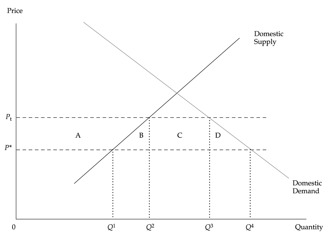
Price P* → Pt, Import Q1~Q4 → Q2~Q3
Consumer loss: - (A+B+C+D)
Producer surplus: +A
Tariff Rev / quota rent / gov gain: +C
National welfare deadweight loss: -(B+D)
** May increase if large country
Quota: Restriction of Q imported w Q set thru import license
Quota rent / profit captured by domestic OR foreign gov: C
National welfare loss: -(B+D+C)
National welfare of foreign country captures quota rent by auctioning import license: -(B+D)
** May increase if large country
Voluntary Export Restraints (VER): Quota / trade restriction by exporting country → ↓ imported goods → ↑ import good price → VER affects / benefits foreign country → greatest welfare loss for importing country bc domestic pays more for same product
Capital restrictions: controls placed on (1) foreigners’ ability to own domestic assets (2) domestic residents’ ability to own foreign assets. Limits the openness of financial markets
Trading bloc / Regional Trading Agreement (RTA):
Free Trade Area (FTA): Free movement of G&S
Customs Union: FTA + common trade policy for non-members
Common Market: Customs Union + free movement of factors of production
Economic Union: Common Market + common economic institution, policies
Monetary Union: Economic Union + common currency
Others:
7. Capital Flows and the FX Market, 8. Exchange Rate Calculation
Exchange rate:
Nominal / Spot exchange rate: Sd/f
= Price / Base = cost of 1 unit of base currency in terms of price currency
= A/B = number of units of currency A that 1 unit of currency B will buy
= USD/EUR exchange rate of 1.17 = 1 euro will buy 1.1700 US dollars = 1 euro costs 1.1700 US dollars, direct quote for European citizens
Nominal adjusted for inflation, assess changes in the relative purchasing power of one currency compared with another
Uses Direct quote d/f
Purchasing power parity (PPP): LT equilibrium of nominal exchange rates
A wants to purchase from foreign country B. A buys fewer goods if nominal spot exchange rate for foreign currency appreciated / foreign price level increased. ↑ real exchange rate = ↓ foreign goods purchasable, ↓ A’s relative purchasing power compared to B
S (Nominal) does not affect Purchasing power
Sd/f × Pf = Foreign price level in domestic currency
Ex) British wants to buy EUR goods [GBP as Price, not base]
Real exchange rateGBP/EUR = SGBP/EUR * (CPIEUR/CPIGBP)
Nominal spot exchange rate GBP/EUR ↑10%, EUR price level ↑%5, UK price level ↑%2
Change in real exchange rate = (1+10%) * [(1+5%)/(1+2%)] -1 = 13%
Real exchange rate ↑13%, costs more to buy EUR goods
== ↑ real exchange rate, ↓relative purchasing power
If Real exchange rate =↑ 5%, Real purchasing power ↓5%
Market participants
Sell side: large FX trading banks (Citigroup):
Buy side: Those using sell side undertake FX transactions. Includes: Corporate accounts (cross-border purchase / sales of G&S, investment), Real money account (unleveraged funds managed by insurance / mutual fund / pension / endowment / ETF), Leveraged account (leveraged professionals managed by hedge funds / proprietary trading shop / commodity trading advisors CTA / high frequency algorithmic trader / proprietary trading desks at banks), Retail, Gov (military purchase), Central banks (influencing domestic exchange rate), Sovereign wealth funds (SWF, gov entities for investmentpurpose rather than public policy)
Market products: FX swaps (Spot + forward FX transaction), Spots (immediate delivery), Forwards (customizable future delivery vs futures), Option
Quotation
Bid: price bank buys currency
= number of units of the price currency client receives from dealer for 1 unit of base currency
Offer: price bank sells currency
= number of units of the price currency client sells to dealer for 1 unit of base currency
Ex. CHF/EUR = 1.1583 - 1.1585:
Client receives CHF 1.1583 (Bid) for selling EUR1
Client pays CHF 1.1585 (Offer) to dealer to buy EUR 1
Dep of A 10% relative to B, (1/1-0.10)-1 % relative to A
% Appreciated exchange rate = % Appreciation of base currency * initial exchange rate
Appreciation of A against B = expected spot / spot -1
Currency regimes:
Ideals: (1) Credibly fixed exchange rate - no currency related uncertainty, (2) Fully convertible currencies - unrestricted capital flow, (3) Fully independent monetary policy.
Regimes: Independently floating rates, Fixed parity with crawling band,
No legal tender: (1) Dollarization, (2) Monetary union (EUR)
Currency Board System (CBS): domestic only issued w foreign currency reserves against the domestic monetary base. Bank is not lender of last resort. Best if (1) wages flexible, (2) non-traded sectors are small (2) global supply of reserve asset grows at a slow, steady rate consistent with LR growth, stable prices. Can earn seigniorage - profit by paying little / no in on its liability (monetary base) to earn market rate on its asset (foreign currency reserves). Ex. HKD
Fixed parity: Currency pegged at currency / basket with (1) no legislative commitment to maintaining parity, (2) target level of foreign exchange level optional
Target zone: Fixed parity w larger band: more freedom / discretion in monetary policy
Active / passive crawling peg: Pegs against single currency, updated periodically
Fixed parity + Crawling bands
Managed / dirty float: Rate based on target policy
Independently floating rates: Rate based on market
Trade balance:
X − M = (S − I) + (T − G),
X = Exports,M = Imports
S = Private Savings, I: Investment
T: Taxes net of transfer, G: Gov expenditure
Investors anticipate change in exchange rate → Sell currency expected to depreciate, buy currency expected to appreciate. Asset prices, exchange rates adjust so potential flow of financial capital is mitigated, actual capital flow remains consistent w trade flow. Thus, capital flow (potential + actual) determine exchange rate movements in ST to intermediate term
In order to stop capital flight (foreign investment in liquid domestic asset suddenly decrease), restrict foreign investment in liquid domestic asset & encourage foreign direct investment.
Forward rate calculation: (indirect format)
In Derivative : 4. Arbitrage, Replication, Cost of Carry in Pricing Derivatives
8. Exchange Rate Calculation
Forward rate calculation: (indirect format)
*** Sf/d × (1 + Forward points as a percentage) = Ff/d
** Ff/d / Sf/d = 1+ rfτ1+rdτ : Forward Premium for base currency (F > S) if int rate in price currency > base currency (rf > rd)
Portfolio Management I
1 ~ 2. Portfolio Risk and Returns
Two Risky Assets Calculation for Return & Variance
Portfolio Return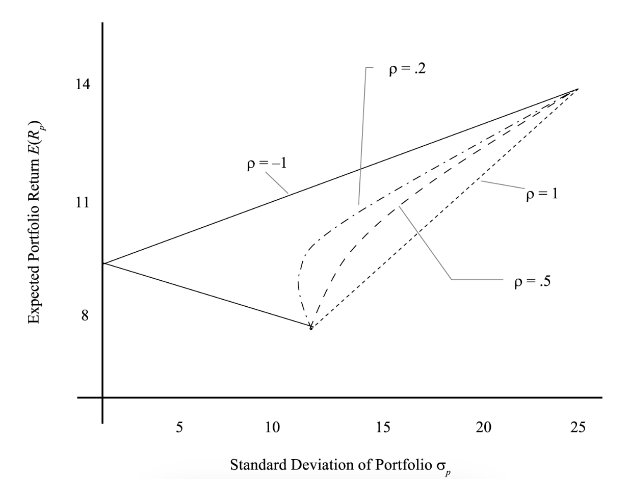
Rp = i=1nwiRi, i=1nwi = 1
If 2 assets,
E(Rp) = w1R1 + (1-w1)E(R2)
Portfolio variance
ρ -1~1
If ρ = 1, no reduction in risk
If ρ <1, little bit of diversification perks
If ρ = -1, portfolio can be made RF
Multiple assets:
σP2 = σ bar 2N + N-1N Cov bar
Where σ and Cov bar are average
= As ↑ N in equally-weighted portfolio, ↓ contribution of each individual asset’s variance to volatility of portfolio.
If N is large, Cov has largest impact on variance
Indifference Curve: combinations of risk–return pairs investor would accept to maintain given level of utility
Utility Theory:
U = E(r) - 12Aσ2
Definition: Measure of relative satisfaction from consumption of various G&S / portfolio
Expected return OR negative term based on the portfolio risk weighted by risk aversion
Conclusions: (1) utility unbounded on both sides (2) higher return = higher utility (3) , higher variance reduces utility, reduction amplified by risk aversion coefficient (4) utility ≠ satisfaction
Loving: exponential, Neutral: linear, Aversive: logarithmic
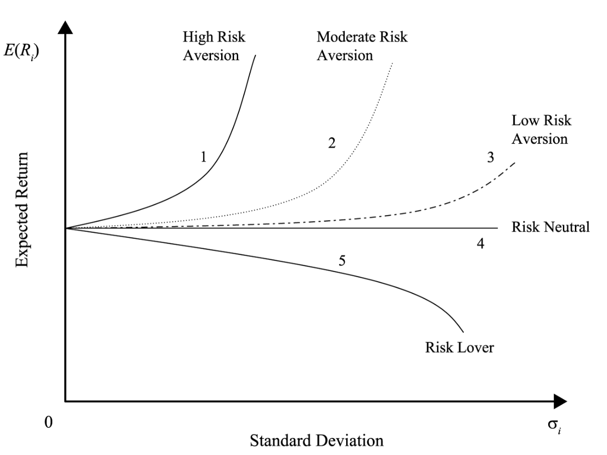
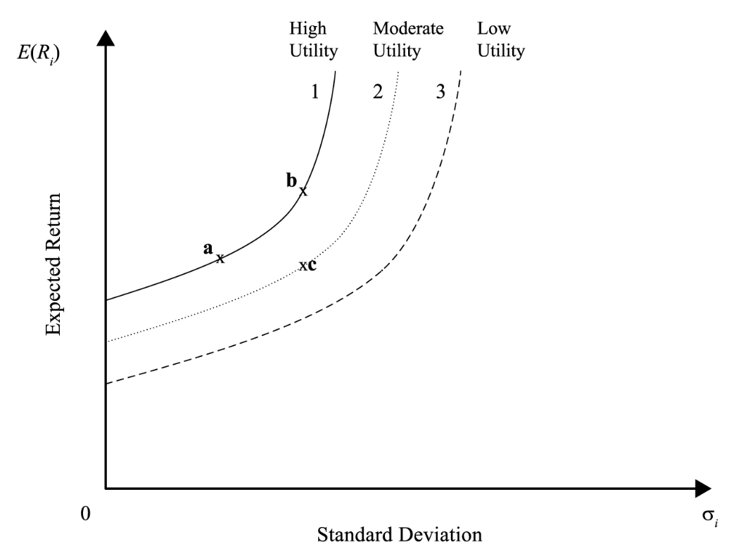
Different Indifference Curves Different utilities for risk aversive indiv
Capital Allocation Line (CAL): portfolio of risky assets + RF assets
E(Rp) = Rf + E(Ri)- Rfσiσp
RF asset has 0 risk, return Rf
Risky asset has σi risk, expected return E(Ri)
E(Rp) = w1Rf + (1-w1)E(Ri)
σp = (1-w1)σi
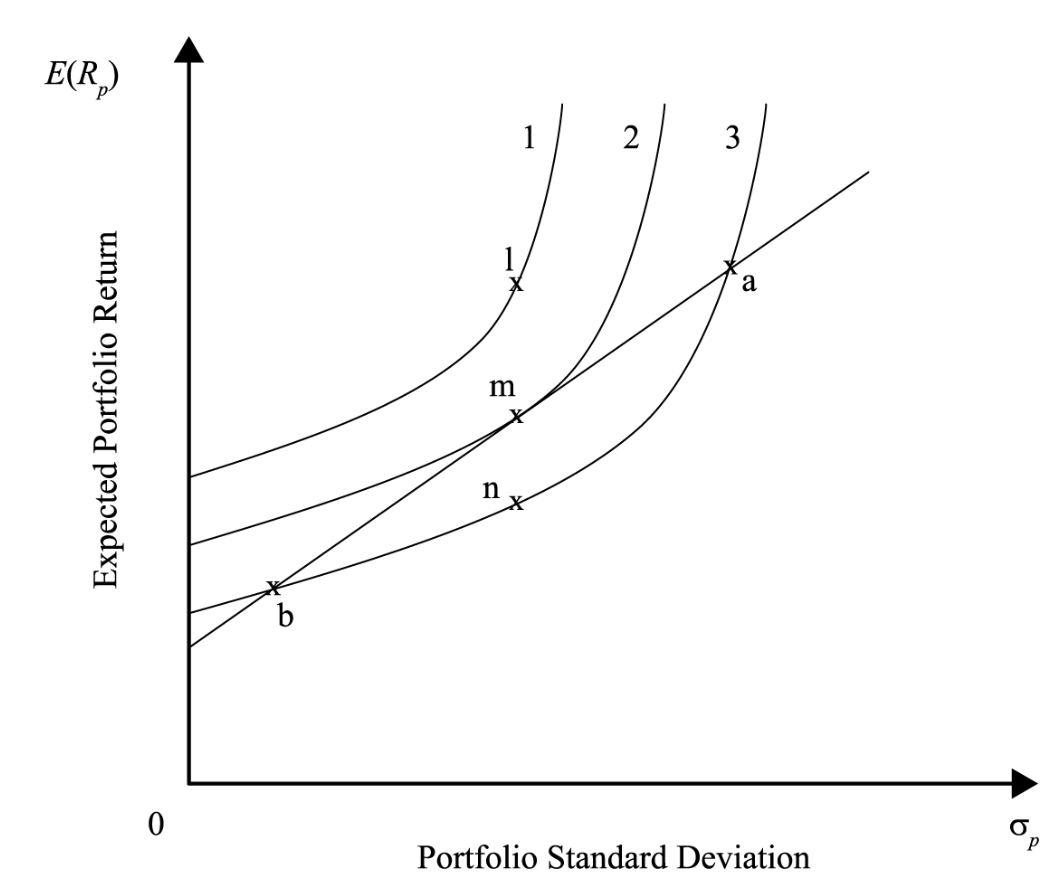
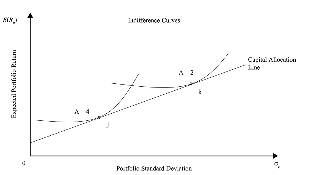
Different Utilities of 1, 2, 3 for high aversive Different Risk Aversions of A = 2, 4. 2 has higher expected return
Efficient / Min Variance Frontier of Risky Assets: min var achievable for given level of expected return
Global Minimum Variance Frontier: portfolio of lowest possible portfolio volatility for a number of underlying assets
Markowitz efficient frontier: Portfolio of risky assets w highest expected return for a given level of risk OR lowest amount of risk for a given level of return. Global min variance frontier ~ up / right. 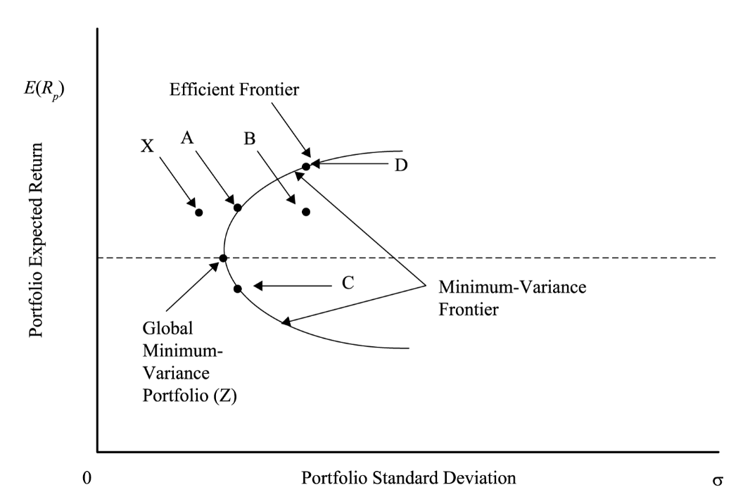
CAL + Efficient Frontier
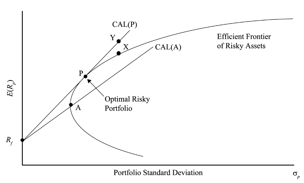
CAL (P) = dominant CAL combining RF asset + optimal risky asset portfolio
It has higher rates of return for levels of risk because of the investor’s ability to borrow at RF rate
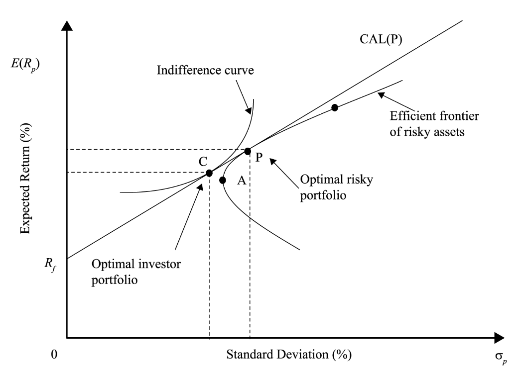
CAL + Efficient Frontier + Indifference Curve
Optimal Risky Portfolio = CAL + Efficient Frontier
Optimal Investor Portfolio = CAL + Indifference Curve
CML: Line w intercept as RF, tangent to efficient frontier of risky assets. RF + market portfolio (risky assets)
CML w dif lending rates:
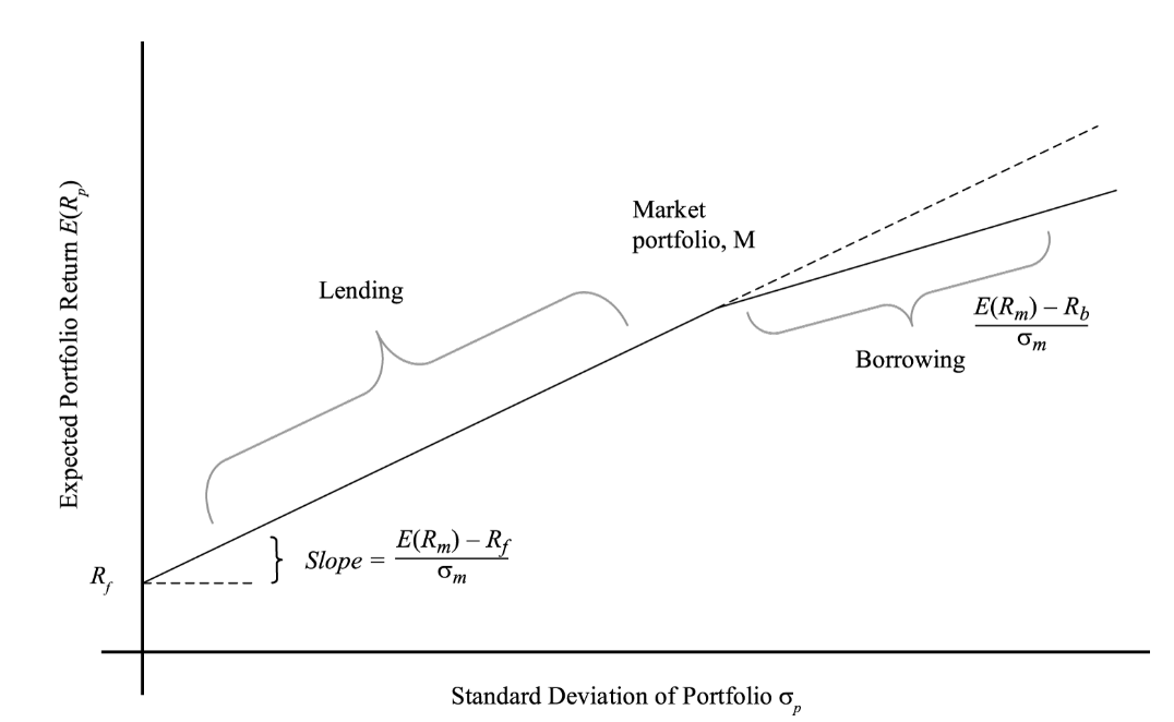
When w1≥0 (lending), E(Rp) = Rf + E(Rm)- Rfσmσp
When w1<0 (borrowing), E(Rb) = Rf + E(Rm)- Rbσmσp
Return Generating Model: Model providing estimate of expected return of security given certain parameters
For Single-Index Model,
E(Ri) - Rf = βi [E(Rm) - Rf]
For Market Model,
Ri = αi + βiRm + ei
Fundamental factor model: bases on earning growth, CF generation
Total variance = Systematic β variance + Nonsystematic variance
σi2 = βi2 σm2 + σe2
Systematic / non-diversifiable / market risk β: risk affecting entire market / econ. According to Capital Market Theory, Systematic risk is priced
Nonsystematic risk: risk to single comp / industry
Covariance dropped bc any non-market return is uncorrelated with the market
βi: Measure of how sensitive an asset’s return is to the market as a whole, market / systematic risk
= Cov(Ri, Rm)σm2 = ρi,m σiσm
Market weight of portfolio: total $ / owning $
Capital Asset Pricing Model (CAPM): E(Ri) = Rf + βi [E(Rm) - Rf],
Assumptions:
Investors are risk-averse, utility-maximizing, rational individuals
Markets are frictionless- no transaction costs / taxes
Investors plan for the same single holding period
Investors have homogeneous expectations / beliefs - allows for the existence of the market portfolio
All investments are infinitely divisible
Investors are price takers
Security Market Line (SML): CAPM on graph
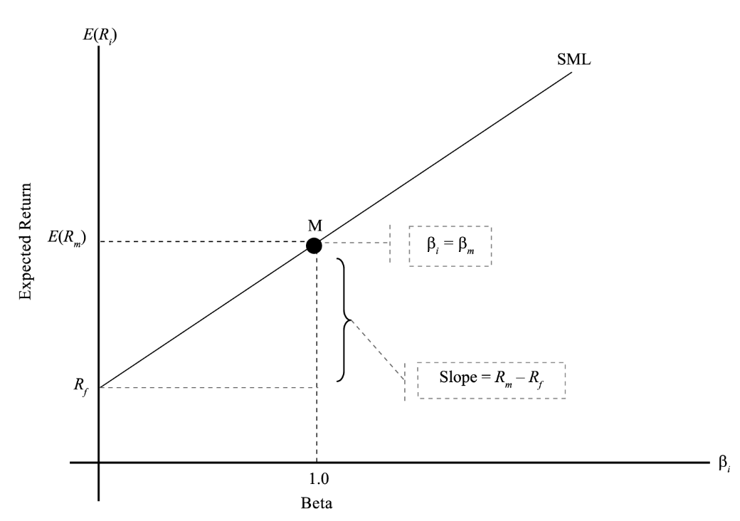 (Above SML: Undervalued / Under SML: Overvalued)
Slope: R m-Rf or [E(Rm) - Rf]: Market risk premium
Portfolio beta = w1β1 + w2β2
Above SML: Undervalued, Under SML, overvalued.
* CAPM finds the Require Rate of Return, E(Ri), which is the amount justified according to its risk within CAPM model. If the ROR < Expected return, it lies above SML, and position shows that security offers a greater return against its inherent = risk is undervalued
Limitations: Single factor / period model, Market portfolio (noninvestable assets), Proxy for market portfolio, Estimation of Beta risk, Poor predictor of returns for CAPM, Homogenigy of investor expectation
Security Characteristic Line:
Ri - Rf = αi + βi (Rm - Rf)
Excess return of a security on the excess return of the market
From Jenson’s αp = Rp - {Rf + βp [E(Rm) - Rf]}
heterogeneity in beliefs of investor, but they are price takes
Jensen’s alpha is the intercept and the beta is the slope.
Performance Evaluation: Measurement / assessment of outcomes of investment mngmnt decisions
** When portfolios are fully diversified, only systematic risk matter
Sharpe / Reward-to-variability Ratio (SR)
= [E(Rm) - Rf] / σp = Risk premium / risk
Excess return per unit of risk. Similar to CAL slope
Adjusts Total Risk, which is for portfolios not fully diversified
Justified ex ante/ post basis
High Sharpe ratio = best risk adjusted performance
Limitations: (1) Adjusts for Total Risk when only systematic is priced, (2) Comparative only (3) Must be positive numerators- neg → incorrect rankings
Treynor Ratio (TR)
= [E(Rp) - Rf] / βp
Excess return on investment w no diversifiable risk
Uses systematic risk beta, which is for fully diversified portfolio
Justified ex ante/ post basis
Limitations: Comparative only (2) Must be positive numerators- neg → incorrect rankings
M2 : Risk Adjusted Performance (RAP):
= [E(Rp) - Rf] σmσp + Rf = SR * σm + Rf
Adjusts Total Risk risk using Standard Deviation to reflect std dev of market, which is for portfolios not fully diversified
Shows what portfolio wouldve returned if it took on total risk as market index. Compare return premiums of adjusted VS market index portfolio
Jenson’s Alpha αp:
= Rp - {Rf + βp [E(Rm) - Rf]}
(actual portfolio return) - (calculated risk-adjusted return) = Abnormal return over the theoretical expected return. Measure of portfolio’s performance relative to market portfolio
αp > 0: Outperform market
Justified ex ante/ post basis
Uses systematic risk beta, which is for fully diversified portfolio
Portfolio Management II
1. Portfolio Management, 2. Portfolio Planning and Construction, 3. Behavioral Biases of Individuals
Basics:
Diversification ratio: SD of equally weighted portfolio / SD of randomly selected security
Portfolio reduces risk more increasing returns
Investment needs: Bank has highest need for liquidity, Endowment has longest term
When defining asset class, (1) assets within a specific asset class have high paired correlations and low correlations with other asset classes. (2) mutually exclusive, add up to approximation of relevant investable universe
Tactical Asset Allocation: deliberate deviation from IPS
IPS Process:
Planning Step: Understanding the client’s needs, Preparation of an investment policy statement (IPS)
Execution Step: Asset allocation, Security analysis, Portfolio construction
Feedback Step: Portfolio monitoring and rebalancing. Performance measurement and reporting
IPS Specifics: Introduction, Statement of purpose, Statement of duties and responsibilities, Procedures, Investment objectives / constraints / guidelines (“distinctive needs”), Evaluation and review, Appendices (strategic asset allocation, rebalancing policy)
Asset mngmnt:
Buy-side: investment mngmnt comp using services of broker dealer
Sell-side: broker/dealer selling security, research, recommendation
Mutual fund: commingled investment pool where investor in fund have pro-rata claim on income / fund value
Open-end fund: trade at NAV, have capital gain distributions
Close-end fund: have capital gain distributions
No-load fund: no fee for investing / redeeming fund share, annual fee based on % of fund NAV
Load-fund: Annual fee + % fee to invest in fund / redemptions
ETF: do not have capital gain distributions
Risk & Return:
Absolute risk: variance / standard deviation, value at risk (money measure of min value of loss expected during time at X probability)
Subjective risk: tracking risk / error (std dev of dif btw portfolio return / benchmark return)
Behavioral Finance:
Illusion of control (over uncontrollable): restrict model to imp variables
Conservatism: review flexible model regularly
Representativeness bias (classifying w standard, not comp specific): Result in under-diversified portfolios. take both into perspective
* Base rates: attributes of reference class, neglect would ignore it in favor of other opinion
Base rate neglect, sample size neglect
Confirmation bias: Result in under-diversified portfolios. incorporate other opinions, seek guidance
Hindsight bias: “history was predictable”
Anchoring / adjustment bias: relying on prev to judge next
Mental accounting bias: looking at everything singularly rather than synergy
Framing bias: asking framed questions
Availability bias: near me
Risk aversion: sensitive to loss than gain thus show disposition effect (investor reluctant to dispose of losing investment, sell when gain too quickly = inefficiency)
Overconfidence: share all forecasts, scenario analysis. “Don’t confuse brains with a bull marke / bubbles” to reduce self-attribution, halo-effect (good now, may make good decision on something else later), ST over incentivization may lead to bubble
Self-control bias: forget ab LT goals bc ST
Status-quo bias: do nothing
Endowment bias: more value when asset owned
Regret-aversion bias: do nothing bc fear regret
4. Risk Management
** Establish risk tolerance → risk budgeting → risk exposure
Risk mngmnt: Process where org / indiv establishes defines / measures lvl of risk to be taken and adjusts to maximize comp or portfolio’s value / indiv’s overall satisfaction / utility. Comprises all decisions / actions needed to best achieve orgal / personal objectives while bearing tolerable risk level
Framework: Risk governance, Risk identification / measurement (quant / qual assessment), Risk infra (database - Risk identification, measurement, monitoring), Defined policies / processes, Risk monitoring / mitigation / management, Communications, Strategic analysis / integration
Good risk governance: Top-down guidance which directs risk mngmnt activities to support overall enterprise. Governance proceeds enterprise wide (not in isolation), determines org’s risk tolerance / provide max loss org can absorb
Factor to be considered: competitive position
Factors not considered in risk tolerance: personal motiv / belief / agenda of BOD, comp size, market environment stability, ST pressure, mngmnt compensation
Risk budgeting: how and where risk is taken and quantifies / allocates tolerable risk by specific metrics
Risk types:
Financial risk: Risk from comp’s capital structure like lvl of debt. Includes Market, Credit, Liquidity risk
Non-financial risk: Risk from external financial market change like accounting rule / legal environment / tax rate change. Includes settlement risk (default risk when settling payments before default), legal risk (sued, contract not upheld by law), compliance risk (regulatory, accounting,tax risk), model risk (wrong model), tail risk (outlier), operational risk (terrorism, WC), solvency risk (bankruptcy)
Risk measuring:
Market risk: SD (not for non-normal, overestimates risk), beta (market risk), value at risk (VaR, tail size to find min loss expected, sensitive to inputs), CVar (Conditional VaR to find max loss expected, can understate risk) scenario loss, delta (small changes in deriv), gamma (large changes in deriv), vega (deriv’s underlying), rho (int for deriv), duration (sensitivity to int). Means thru scenario analysis, stress testing (loss in scenario analysis)
Credit risk: liquidity / solvency / profitability / leverage, strength / cyclicality of macro / industry. Ex. Credit VaR, prob of default, expected loss given default, prob of credit rate change
What to do with risk:
Risk acceptance: bear risk, self-insurance by setting reserve fund to cover loss, diversification
Risk transfer: insurance = surety bond
Risk shift (change distribution): use deriv (forward & contingent claim)
Corporate Issuers
Business Structures:
Governance:
During legal claim, stakeholder (debtholder) → creditors (int /principal), supplier (account payable), gov (tax), employee (wage) → shareholder (Equityholder)
Equity: loss limited to equity investment
Climate change considerations: (1) physical risk - climate risks that may be insured / diversified (2) Transition risk- transition to lower carbon. Ex. stranded assets (unviable asserts)
Stakeholder conflicts:
Principal - Agent (agency) relationship: principal hiring agent to perform task
Managers interest can diverge (1) insufficient effort (2) inappropriate risk appetite (3) empire building (4) entrenchment - retain job (5) self-dealing - corruption
Debtholders prefer equity raising to limit SH distribution, SH prefers greater leverage. SH distribution than dilutive equity
SH meetings:
Annual General Meeting (AGM): board member elections, independent auditor appointment, FS / dividend director auditor compensation approval, nonbinding vote on compensation plan
Extraordinary GM: special board member election proposed by SH, bylaw / article amendments, M&A / takeover / asset sales, capital increase, voluntary firm liquidation
SH activism protects interest by increasing SH value. May lead to litigation / lawsuit: proxy contest (group persuading SH to vote for group), tender offer, hostile takeovers. Comps can defy with SH Rights Plan / poison pills
Creditors (bondholder / private lenders) protects interest by bond indenture (contracts), creditor / ad hoc committees
Audit committee: Monitors financial reporting process (selection / implementation of accounting policies), supervises internal audit function / independence / competence, recommends independent external auditor and proposing its remuneration
Working Capital Liquidity:
Operating Cycle: Company’s acquisition of goods / raw materials ~ collection of cash from sales.
Cashflow may not happen at same time as activity
Inventory: Cost of products produced or purchased for sale
Recognized when issuer takes ownership of materials, goods, supplies
Derecognized when product is sold to customer
Account Receivable (AR, BS ST asset): $ to be collected for products sold.
Account Payable (AP, BS ST liab): $ owed to suppliers for products received
Recognized when product is received, issuer defers / delay payment to supplier
Derecognized when cash is paid to supplier
**2/10 net 30 : 2% discount if account paid within 10 days, and otherwise full amount due in 30 days
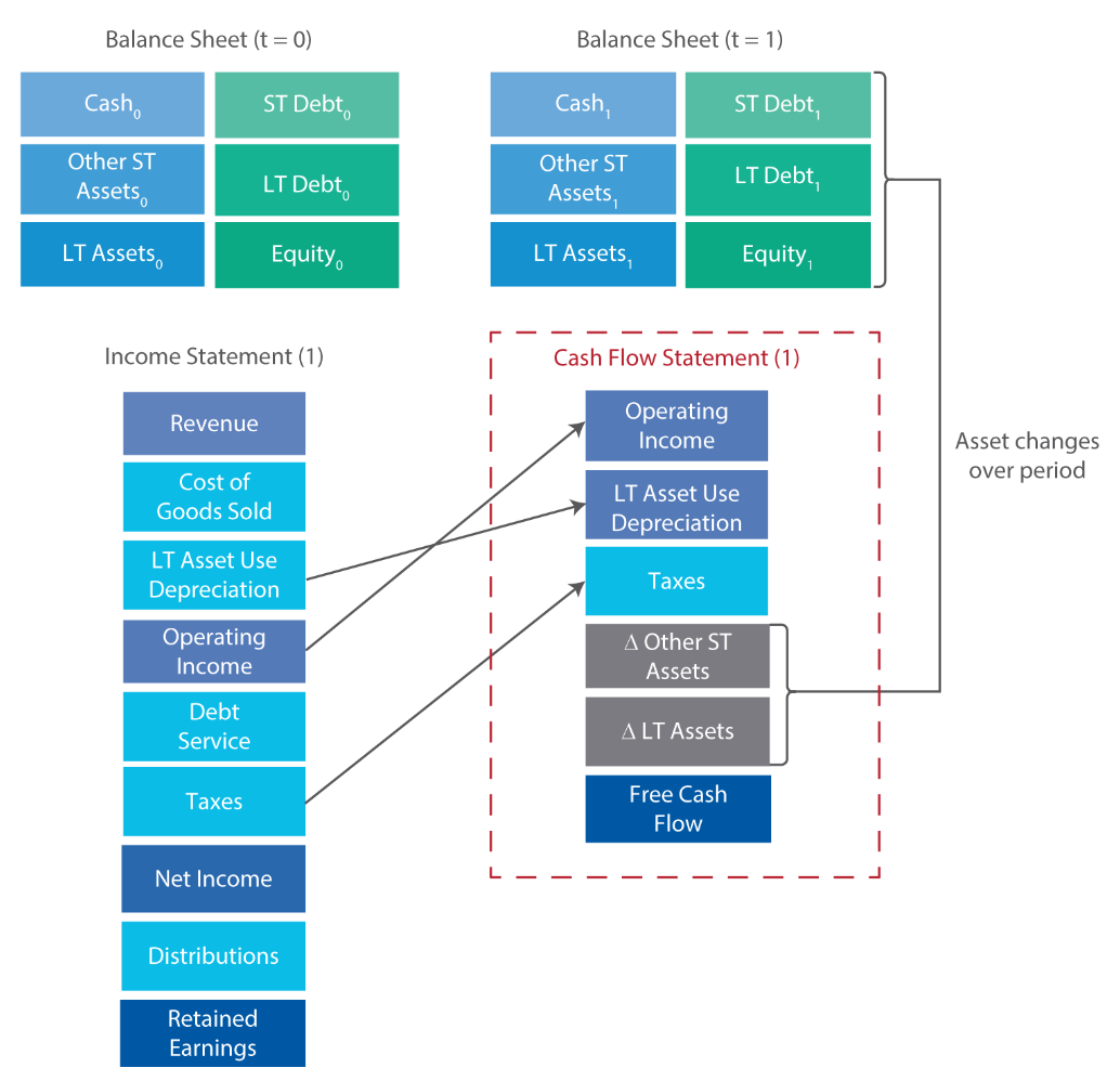
Secondary Liquidity: (1) suspend / reduce div for SH (2) delay / reduce capital expenditure (3) issuing equity (share issuing provides cash but dilutes exiting SH cost) (4) renegotiation contract terms (ST debt, debt covenants) (5) selling asset (6) bankruptcy
Factors affecting Liquidity:
Drag on liquidity (inflow): event reducing available funds / delays cash inflows
Uncollected AR: Measured by av # of days receivables are outstanding, level of customer payment delinquencies as a percentage of receivables
Obsolete (out of date) inventory: If finished goods held too long in inventory, may mean no more demand / products only sold at discount
Borrowing constraints: ST debt more expensive / unavail when credit conditions tighten
Pull on liquidity (outflow): event accelerating cash outflows or trade credit availability is limited, requiring companies to expend funds before they receive proceeds from sales that could offset the liability
Early payments: w out benefits = comp forgoes fund use
Reduced credit limit: when comp pays late often, supplier can cut credit
Limit on ST lines of credit: by bank / gov mandate / market related
Low liquidity positions: liquidity shortage due to industry condition / weak financial position. May be exacerbated w aggressive WC mngmnt (more cash, ST, cheaper)
Capital Investments and Capital Allocation
Capital Investment / Projects:
1~ investments, initially recorded at cost (like most assets)
IS: Expenditure not recorded, Non-cash dep / amort over asset life recorded
BS: Expenditure recorded, Subsequent periods presents net basis (cost - accumulated dep / amort) to 0 or salvage value
CF Statement: Cash capital spending reported as incurred
Project types: (1) Going concern / maintenance [operation] (2) regulatory/compliance projects [3rd party required] (3) Expansion (4) Other [high risk new initiative]
Capital Allocation - Investment analysis (time-value-of-money concepts.)
= PV of investment CF inflow - PV of CF outflow
Internal Rate of Return (IRR)
t=0TCFt(1+IRR)t = 0
= Disc rate making NPV = 0
Required Rate of Return = Hurdle Rate: Preferred / min return return on investment that a fund must reach before a GP receives carried interest
Multiple IRRs exist if cash flow signs (+/–) change more than once
Return on Invested Capital (ROIC) or Return on Capital Employed (ROCE)
= After-tax Op ProfittAv Invested Capital = (1-Tax rate) Op profittAv total LT L&E Invested Capitalt-1, t
= After-tax Op profitSales × SalesAv Invested Capital
= After-tax OPM × Capital or Asset Turnover
Av LT liab, equity includes LT D, Share Capital, Retained Earning
Aggregate measure to gauge firm’s ability to create value across all investment
Comparing to ROR, if ROIC > ROR, 🙂
🙁Accounting, not cash-based method, backward looking
If two mutually exclusive project, can only undertake one
Capital Structure
** ** Calculate WACC: Cost of Debt = int cost (=min ROR) VS Cost of Equity = DDM or CAPM
Cost of Capital (COC): WACC
= (Cost of debt × Weighting of debt) + (Cost of equity × Weighting of equity)
= Cost of financing comp = Opportunity cost of fund for suppliers = Required ROR suppliers of capital require as compensation for capital = measured by Weighted Average CC (WACC)
Moldigliani and Miller (MM) Proposition: ??????????????????????
Comp’s choice of capital structure does not affect its value (value = PV of firm’s expected future CF, discounted by its WACC). Future CF is most imp
Assumptions: (1) homogeneous expectations of future earning/CF, (2) Perfect capital market [no tax / transaction cost / bankruptcy cost, symmetric info], (3) RF rate lending / borrowing, (4) No agency cost (5) Independent decisions
V = Market Value
Proposal 1 (w/out tax): Capital Structure Irrelevance:
keep in mind RF lending rate + arbitrage possible,
VL = VU :: Value of levered comp = Value of unlevered comp
Value of comp determined by expected future CF
WACC unaffected by capital structure
Proposal 2 (w/out tax): Higher Financial Leverage Raises the COE:
Proposal 2 (w tax): Firm Value with Taxes:
Profitable company can ↑ value (V) by using debt
↑ tax rate, ↑ benefit of using debt in the capital structure
Proposal 2 (w tax): COC:
Cost of financial distress
VL = VU + tD - PV
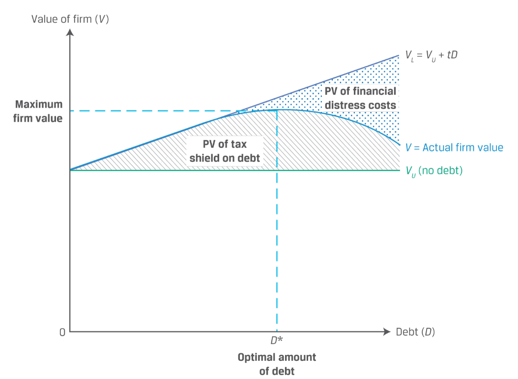
D* maximized firm value, Associated equity = optimal capital structure
static trade-off theory of capital structure: ↑ leverage = ↓ firm value, PV of financial distress > tax benefits
↑ business risk. = ↑ Value-reducing impact of financial distress / bankruptcy
Target Capital Structure: mngmnt’s desired D/E proportion, stated in book value / indirectly using financial leverage metric (net or gross debt to EBITDA, credit rating, etc). This is because market value fluctuates substantially, mngmnt’s concern is amount / type of capital investment by comp (not in comp), policies aligned to measure used by 3rd parties
Example:
Pecking Order Theory: Managers, incorporating consumer views, prefer decisions least visible (internal equity) over most visible (equity)
Business Model
Pricing model:
Simple products: (1) Tiered - dif P for each buyer / volume / product feature (2) Dynamic - dif P for time / customer depending on avail supply ie. hotel (3) Value-based - value /effectiveness received by customer ie. pharmaceutical (4) Auction - bidding
Complex products: (1) Bundling (2) Razor, razorblad pricing - low qual P on initial purchase + high margin on its equipment (3) Add-on pricing - optional service ie. league skins
Penetration pricing: lower price to penetrate market
For digital models: (1) Freemium biz model - certain lvls free (2) hidden rev biz model - ads
Alternatives: (1) Subscription (2) Leasing, licensing, franchising
Biz model:
Contract manufacturer: branded products w manufacturers
Value-added reseller: add customization / installation / support
Licensing: use brand for loyalty
Financial Statement Analysis
Financial Reporting Quality:
Earning quality good = sustainable, FS quality good = well represented
Within GAAP (biased choice) > Within Gaap (EM) > Outside Gaap (conservative choice)
Aggressive = higher income bias
Conservative = higher sustainability of earning
Motivation for low qual FS: (1) beat benchmark (2) career or incentive [unexpected biz strength banked for next per]
Condition for low qual FS: (1) opportunity [poor in/external control, min consequence, gov cutbacks on financial regulator] (2) pressure / motivation [bonus] (3) rationalization
Spectrum of Quality:
GAAP, decision-useful, sustainable, adequate return
Principle-conforming, Decision-useful info [= relevance + faithful representation, Enhancing characteristics (= Comparability, verifiability, timeliness, understandability)]
GAAP, decision-useful, unsustainable
GAAP, biased choice (unintentional): Aggressive / conservative accounting, Earning smoothing (underestimate volatility)
GAAP, Earnings mngmnt (EM = intentional)
Non-compliance accounting
Fictitious transaction
FS Quality Discipliners:
Market Regulatory Authorities
Ex. International Organization of Securities Commissions (IOSCO):
Global standard setter for the securities sector [Technically not a regulatory authority and standard setting]. Thus Establishes objectives and principles to guide securities and capital market regulation
Aims to protect investors, ensure a fair / efficient / transparent market, reduce systemic risk
Promotes cross-border cooperation and uniformity in securities regulation
Ex. SEC: Securities / capital market regulator
Statutes enforces include ① Securities Act of 1933 (registration of all public issuance of securities, inform properly), ② Securities Exchange Act of 1934 (create SEC, enforcing periodic reporting and authority over industry), ③ Sarbanes-Oxley Act of 2002 (create Public Companies Accounting Oversight Board, or PCAOB to oversee auditors, addressing auditor independence, enforcing mngmnt / auditor to report effectiveness of internal control)
Regulatory regimes affect FS thru Registration / Disclosure / Auditing requirements, Management commentaries, Responsibility statements, Regulatory review / filing
Standard setting bodies (IASB, FASB): Private sector, self-regulated org w board members as experienced accountants, auditors, academics. Sets standards
Regulatory authorities (SEC): Legally enforce (thru fines, suspending market participants, criminal prosecutions) financial reporting requirements
Auditors: Unqualified - Qualified - Adverse - Disclaimer of opinion
Private Contracting: Loan agreement covenants
FS Issue Detection:
Can inflate performance thru: recognize rev / expense prematurely / late, use non-recurring transactions to increase profit, adjusting EBITDA [(Rental payments for OL to result in EBITDAR with R as rentals, Equity-based compensation as it is non-cash expense, acquisition related charges, imp charges for goodwill / LLA, litigation cost, debt extinguishment), reduce uncollectible AR
SEC prohibits exclusion of charges or liab requiring cash settlement from any non-GAAP liquidity measures other than EBIT and EBITDA
CFS may improve if (1) increased AP credit period (2) not applying non-cash discount amort against int capitalized [= lower cash outflow] (3) Shifting classification of interest paid from CFO to CFF
Channel stuffing: Overloading distribution channel w more product than it is normally capable of selling. Overstates my revenues, AR (corrected when product is returned next period), understates my inventory in current period
Premature rev recognition - ↑ DSO
CFO / NI < 1.0. If not, may be aggressive accrual accounting policies
If large restructuring charge in earning, make pro forma adjustments to prior years’ earnings to reflect those prior years a reasonable share of current period's restructuring / imp charges
FS Example Files used for Financial Analysis:
Common: ① Securities Offerings Registration Statement (1933 Act - required info includes disclosures of securities being offered, relationship of new / other securities, annual filings info, recent audited FS, risk factors), ② Form 10-K, 20-F, 40-F (full required annual FS files for US SEC / CAD / non-US registrants. 10-K includes footnotes, MD&A, auditor’s report) ③ Annual report (comp annual report for investors, not required by SEC), ④ Proxy Statement / Form DEF 14A (Proxy required by SEC, info for casting votes once a year - proposals requiring SH vote, security ownership details, biographical info of directors, executive compensation ⑤ Forms 10-Q and 6-K (interim files, including unaudited FS, Management Discussion & Analysis, or MD&A, nonrecurring events)
Footnotes (in 10-K):
Basis of preparation for FS: accounting policy / method / estimates, unit, rounded minor discrepancies (cost allocation of dep), consolidated basis, segment reporting, biz acquisition or disposal, contractual obligations, financial instruments and its risks, legal proceeding, related party transaction
Operating segment: Part that needs disaggregated full FS. Part that engages in activities that generate rev / create expense, which results regularly reviewed by senior mngmnt, which discrete financial info is avail
Comp must disclose all Operating segments that constitute 10% or more of combined operating segments’ rev / asset/ profit. Segments must [segments for 75% of total comp rev]
75% of total comp rev must be reported, including operating segments and others
Each reportable segments must include: rev, measure of profit / loss / asset / liab, interest rev / expense, cost of PPE / intangible assets required, dep / amort expense, other on-cash expense, income tax expense / income, share of net profit / loss of investment accounted for under equity method
MD&A (Management Discussions & Analysis or Management Commentary, in 10-K):
Includes: nature of the business, past results, outlook
Unaudited
IASB framework: “decision-useful mngmnt commentary”: (1) nature of biz (2) mgnmnt’s objectives / strategies; (3) comp’s significant resources, risks, relationships (4) results of operations (5) critical performance measures
SEC requirements: un/favorable trends, significant events, uncertainties affecting comp liquidity / capital resource / operation results, effects of inflation, changing P, off-balance-sheet obligations, contractual commitments (purchase obligations),
Issuer sources: Earning call, press release, interviews, comp website
Public 3rd party source: Industry whitepaper / analyst report, economic indicators from gov, news, SNS
Proprietary 3rd party source: analyst report (credit rating), Platform reports / data (Bloomberg) / consultancies
Proprietary primary research: survey, product comparison
FS Analysis Framework
Articulate analysis’ purpose / context:
Thru evaluation, communication, and guidelines,
Produce analysis’ objective, target Q, reporting contents, timetable / budget
Collect input data:
Thru FS / questionnaires / data, discussion w related parties, comp site visit
Produce organized FS, questionnaires
Process data:
Thru data,
Produce adjusted FS, common size statements, ratios, graphs
Analyze/interpret the processed data
Thru input / processed data (including ratios),
Produce analytical results, forecasts, valuations
Develop / communicate conclusions / recs in analysis report
Thru analytical results / prev reports, institutional guidelines,
Produce report answering target Q, recommendations
Follow-up
Thru periodically gathered info / repetition,
Produce comparison of actual / expected results, revised forecasts, updated report / suggestions
FS Modeling:
IS: Forecast for: Rev → Op Expense (COGS, SG&A) → Pro Forma EBIT (Segments forecast check) → Non-op Expense (Int exp, Inc tax, Shares outstanding) → Pro Forma IS
CFS: (CFO) NI, Shared based compensation, WC, Dep & Amort. (CFI) CAPEX. (CFF) Share repurchase & issuance, Div, Debt issuance & Repayment
FS Analysis types:
Sensitivity analysis: what-if, assumption changed
Scenario analysis: Key financial Q changed
Simulation: Computer-generated sensitivity / scenario analysis based on probability
Incorporating Competitor impacts: Porter’s Five Force model finds relative profit potential of comp. Includes industry competition, Potential for new entrants, Supplier power, Customer power, Substitute product threat
Incorporating In/deflation:
Industry sales: ↑ P / inflation may have bad impact on volume if Demand is Price Elastic, cheaper substitutes avail. ↓ P may also start downward price competition
Comp sales: ↑ impact:
∆%Revenue = (1+ ∆%P for rev)(1+∆%Volume) -1
∆%COGS = (1+∆%Volume)(1+∆%Input cost) -1
Total Rev - COGS = Gross Profit
Financial Statements : IS, BS, CFS
1. Income Statement, Statement of comprehensive income / operations, P&L
Financial performance as flowing statement
General principle: Accrual accounting - Rev recognized / reported on IS when earned, so comp’s record reflect rev from sale when risk and reward of ownership is transferred
Converged accounting standards (IASB + FASB) May 2014: Aims to provide principle based approach to revenue recognition
* Incremental costs of obtaining contract / certain costs incurred to fulfill a contract must be capitalized
Revenue recognition:
Framework: (1) identify contract w customer (2) identify distinct performance obligations in contract, (3) determine transaction price (4) allocation transaction price to performance obligation in contract (5) recognize rev when entity satisfies performance obligation
(2) G&S is distinct if customer can benefit from it / promist to transfer can be separated from other promises
If Rev may not be recognized, record minimal amount of Rev upon sale, recognize refund liability and “right to returned goods” asset on BS as carrying amount of inventory - cost of recovery
(5) transferring control of G&S is when entity has present right to payment, customer has legal title / physical possession / significant risk & reward of ownership / accepted G&S
** Net Rev: Rev for goods sold - return, allowances, discounts
Examples: Pizzahut
Selling own food:
+ Sales for selling food
- Cost of sales to make food
Selling food as agency made by others:
+ Sales for agency fee
Franchise royalties: (gives others license to operate)
+ Rev for franchise royalty (not Sales)
- Upfront fee for opening new unit as Def Rev (amortized to Rev in SL basis)
Selling license for tech they invented:
Rev recognized over time of license if
Seller continues to undertake activities (upgrade / enhancements)
Customers are positively / negatively impacted from those activities
Activities don’t result from transfer of G&S
If not, rev recognized at beginning when license is transferred
Selling LT contract: recognized over time if 1 of below conditions are met:
Customer routinely benefits
Entity’s performance creates / enhances asset enhances asset
Entity’s performance does not create alternative use
Bill and hold arrangement: billed but holding for reason (ex. can’t move equipment yet / storage issue) if all of below is met
Reason for arrangement is substantive (customer asked for it)
Product identified separately to belong to customer
Product ready for physical transfer to customer
Entity can not use product / direct it to another customer
Selling at gallery through consignment basis: Rev recognized when gallery sells. Risk and reward is transferred and Rev is measurable
Selling when collectability concern: Rev recognize when remits payment for the pizza
Selling to 3rd party directly: Rev recognized when receives the pizza
Service Rev: Rev recognized as completion of work ie. construction
Expense Recognition: (Capitalizing VS Expensing)
Recognition models:
Matching principle: Expense recognized at the same period when associated revenues from sale of goods are recognized
Expensing as incurred: Period costs are costs that can not be directly matched with the timing of rev, thus are expensed immediately ie. executives’ salaries
Capitalization with subsequent dep or amort:
First, expenditures capitalized on BS (Asset), and CFS (investing cash outflow)
Later, comp expenses the capitalized amount over asset’s useful life as dep or amort expense (excludes nondepreciating assets like land, unamortzable assets like intangibles w indefinite life). Expense ↓ NI on IS and ↓ assets on BS. Bc dep and amort are non-cash expenses, so no impact on CFS (excluding impact on taxable income, taxes payable)
Expenditure:
Capitalizing: ST 🙂:
Beg years:
↑ NI, profitability, profitability ratios (ROE, NPM), BV for assets (Costs recorded as Asset on BS then depreciated), taxable income (expense is smaller) and tax paid,
↓ expense, CFO (if higher taxes paid), total asset turnover (Sales / Total Assets bc assets are bigger)
** Overall: ↑ CFO as long as capital expenditures > dep expense
Interest cost: either capitalized (on BS) or expensed (IS)
Internal Development Costs:
Capitalize after product’s feasibility is established, reported as CFI outflow
If expensed,
↑ Net CFI, market multiples
↓ Operating income, EPS, CFO (by CFI outflow), historical profits, EBITDA
↓ NI as long as (current development expense > amort expense that would have resulted from amortizing prior period’s capitalized development costs), = usually when comp’s development costs are increasing
No amort of prior years’ software cost
Comp that capitalizes VS expenses: analyst can adjust a capitalizing comp by
(1) IS - include software development cost as expense, exclude amort of prior years software development cost
(2) BS - exclude capitalized software [decrease asset and equity]
(3) CFO - decrease CFO, cash used in investing by the amount of the current period’s development cost
** EBITDA: include developmental cost and exclude amortization of prior expense
Non-recurring Items: Ex. Restructuring charges (costs to close plants, employee termination) gain / loss from selling comp asset for more / less than carrying value
Changes in Accounting Policy
Income Tax
Carrying Value Standard, Should pay: (IS) Accounting profit or Book Profit = income before tax (EBT or Pretax Income), Income Tax Paid, Reported on FS earning, No provision for Income Tax Expense Accrual basis | Tax Base Actual paid: (BS change) Taxable income / profit, Basis for Income Tax Payable (L) / Recoverable (A - Tax credit), Cash Basis |
Taxable Differences:
Permanent:
Dif w no reverse in future
Treat DTL as
Ex. Div receivable, Donation, Loans, Income / expense items not allowed by tax legislation (Penalties, Fines), Tax credits directly reducing tax (encourage solar power use / EV)
DTA: ↓Accounting profit, amount expensed, ↑Taxable income
DTL 🙁= Pay less tax now, pay more in the future
Calculations:
Tax Expense or Provision (IS)
= Income Tax Payable / Recoverable + ∆ DTL - ∆ DTA
= EBT or Pretax Income × Tax Rate
= tax expense + Δ Tax Expense + Δ Def Tax
NI = EBT or Pretax Income - Income Tax Expense or Provision
∆ NI = ΔDTA - ΔDTL - Δvaluation allowance
EBT or pretax income = Expected income tax expense from continuing operation × Tax Rate
Income Tax Payable = Taxable income × Tax rate
Deferred tax = Temp Dif × Tax rate
Effective Tax Rate = Total Provision for Income Tax/ EBIT
Balance Sheet Item | Carrying Amount vs. Tax Base | Result / Temp Dif Type |
Asset | Carrying Amount > Tax Base | DTL, Taxable Temp Dif (TTD) |
Carrying Amount < Tax Base | DTA, Deductible Temp Dif (DTD) |
Liab | Carrying Amount > Tax Base |
Carrying Amount < Tax Base | DTL, Taxable Temp Dif (TTD) |
Corporate Income Tax
Effective tax rate:
Cash tax rate
Statutory tax rate: Domestic Corporate Income Tax rate
Dif btw Statutory tax rate & Effective Tax Rate can be because Tax credit, Withholding tax on div, Adjustments to prev yrs, Non-deductible expenses for tax purpose, when comp is active outside domiciled country
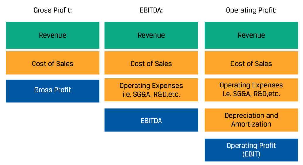
2. Balance Sheet, Statement of Financial Position
Financial position at point in time
Asset Impairment
Impairment: Carrying amount > Recoverable amount (=Carrying amount not recoverable) = Writedown carrying reduces Asset (BS) and NI (IS). Non-cash item
** Impairment loss: insufficient dep expense was recognized in prior years, NI was overstated in prior years. NPM will be higher later
** Impairment write-downs: ↑ D/E Total Asset Turnover (TAT = Rev / Av Total Asset) ↓ Equity, Asset
Current Asset: Inventory
Analysis:
↓ allowance for obsolescence => ↑ cost of sales => ↓ profit margin
Inventory is divided into Cost of sales (sold) and Ending inventory (not sold)
In ↑ inventory unit cost, ↓ inventory quantity
↓ cost of sales (IS)
LIFO
↑ cost of sales (IS), Inventory turnover (efficiency)
↓ ending inventory (BS), profit, gross / op profit / IBT (profitability), Current ratio (liquidity)
* cost of sales similar to current replacement cost of inventory
Current or Non-current Asset: Financial Assets
Recognition can be at:
**
Fair Value: $ that would be received to sell an asset / paid to transfer a liab in an orderly market transaction
Amortized Cost: ($ A/L is initially recognized) - (principle repayments) ± (amort of discount / premium) - (reduction for impairment)
** OCI = (1) Foreign currency translation adjustment (2) Unrealized gain / loss on deriv contracts accounted for hedges (3) Unrealized holding gains / loss on avail for sale debt securities / securities designated as fair value thru OCI (4) comp’s post retirement
Non-Current Asset: PPE:
Impairment
Disclosure:
Measurement basis, Dep method, Useful life (Dep rate), Gross carrying amount, Accumulated dep at beg / end of period, Reconciliation of carrying amount at beg / end period, Restrictions on title / pledges as security, Contractual agreements to acquire PPE
When Revaluation model is used: How fair value is obtained, Carrying amount under cose model, Revelation surplus, Dep expense for period, Balances of major classes of depreciable assets, Accumulated dep by major class / total, General description of dep method used to compute dep expense
Non-Current Asset: LLA:
When LLE is first purchased, ↑ Dep Expense (IS), Asset (BS)
Impairment: LLA Held for Sale:
When Assets are decided to be held for sale, Asset reclassified from (PPE) Held for use → (Non-current Asset) Held for Sale, and tested for impairment. Impaired if (Carrying amount > Fair value - Cost to sell), Asset written down to (Fair Value - Cost to sell). LLA Held for Sale is not dep / amort
Reversal: IFRS vs USGAAP below
Derecognition: Remove from FS when asset no longer provides future benefits from use / disposal
Disclosure: (IFRS)
Nature of expense method: Comp aggregates dep expense according to nature (dep, purchase of material, transport cost, employee benefit, advertising cost..) w no relocation
Function of expense method: Comp classifies dep expense according to function (cost of sales, SG&A..)
Non-current Asset: Intangible Assets
Definition: non-monetary assets without physical substance. Must be:
1) Identifiable: Capable of being separated from entity / arising from contractual or legal rights
2) Under control of comp
3) Expected to generate future econ benefits
4) Probable of expected future econ benefit of the asset will flow in comp
5) Cost of Asset can be reliably measured
Measuring Model:
Assessment:
Finite life: Amortized on systematic basis over best estimate of useful life
Amort method and Useful life estimation reviewed at least annually
Indefinite life: Not amortized
Reasonableness of assuming indefinite life reviewed, Asset tested for impairment
Identifiable Intangibles: Ex. Patent, license, trademark, customer list
IFRS: Assets recognized on BS if probable of future economic benefits, cost of asset is measurable
Internally Created:
IFRS: Research phase (Expensed), Development (Capitalized if tech feasibility met)
USGAAP: Most Expensed, Capitalize SW development w tech feasibility (cost of employee)
Expensed for both: Internally generated brands / mastheads / publishing titles / customer list, start-up / training / admin and overhead / redundancy / termination cost, advertising / promotion, relocation / reorganization expense
As generally expensed, recognizes lower Asset amount than comp obtaining thru external purchase
CFS classified as CFO
Purchased:
Acquired in Biz Combo (not including Goodwill)
Biz combo accounted w Acquisition Method, Acquiree’s Identifiable A&L and Contingent Liabilities measured by Fair Value. Difference between the two = Net Identifiable Assets Acquired
USGAAP: To not be Goodwill,
Item arising from contractual / legal right
Item separable from acquired comp (Exclusive rights: patents, internet domain names, audiovisual materials)
Non-identifiable Intangibles: Goodwill:
Definition: (Net Identifiable Assets Acquire) - (Acquired Company)
Assessment:
Capitalized, Not amortized, Tested for impairment annually
If Goodwill impaired, Impairment Loss charged against Income, ↓ Earnings, Total Assets, ↑ ROA in future periods.
Non-cash Item
Recognition: Goodwill arising from purchase = Cost of comp - Net Identifiable Assets Acquired
Disclosure: Acquisition date Fair Value of the total cost to purchase comp, acquisition date amount recognized for each major class of A&L, qualitative description of goodwill recognized
Disclosure: IFRS vs USGAAP below
Non-current Liabilities: LT Financial Liab
Amort Cost (BS): Loans / Bond Payable
At maturity, Amort Cost of bond (Carrying Amount) = Face Value of bond
Ex. Today: cop, issues $10 bonds at 9.75% of par value (discount) = bonds reported as $9.75 at issue date, discount of 2.75 amortized, bond will report liab of $10 at maturity
Fair Value: Bonds issued by comp held for trading / deriv, non-deriv hedged by deriv
Non-current Liabilities: Lease
Lease: contract conveying right to use in exchange for fee. Contract must (1) identify underlying asset, (2) give customer right to obtain econ benefit from asset over contract term (3) give customer ability to direct how / what asset’s objective is
Lessee = Using asset, borrower, Pays fee = Customer
Similar to acquiring asset w note payable
Lessor = Owns asset, lender, Grants rights for use, Receives fee
Similar to installed payment investment
Advantage
Classification:
Reporting [(Initial Recording) - (Subsequent Recording)]
For Lessee (borrower, fee payer)
IFRS:
Same for FL, OL
BS:
IS: Interest Expense on lease liability, Amortization Expense related to ROU. Reported separately
CFS:
** Lease Payment = Principal Repayment + Interest Expense (Int × Last year Lease Liab)
USGAAP: (FL: Same as above)
OL:
BS:
Lease Payable Liab, ROU: Both initially record PV of future lease payment, [reduce balance of liab by lease payment, recognize Int Expense??]
Subsequently, ROU amort expense = Lease Payment - Interest Expense , [record dep expense]
IS: Lease Expense (Interest expense on lease liab + Amort expense for ROU) single line
CFS: CFO outflow
** Lease Liability = ROU asset (principal repayment and amort calculated the same)
** When using OL (vs FL), ↑ Asset, ↓ EBITDA margin, Asset Turnover, CFO
Disclosure (FL + OL): Carrying amount of ROU asset and end of period by class, Total cash outflow for lease, Int expense on lease liab, Dep charge for ROU by class, Addition to ROU asset,
+ Maturity / quantitative / qualitative analysis: Nature of lessee’s leasing activity, Future CF lessee is potentially exposed to but not reflected, Restriction / covenants, Sale / leaseback transactions
Lessor (lender)
Identical IFRS, US GAAP
Rev = Value of leased asset, COGS = Carrying value of asset
Non-Current Asset: Post Emp, Share-Based Compensation Plans
When employee earns salary / bonus, comp records
However, Def Compensation earns compensation now but receive consideration in future. Ex:
Defined Contribution Pension Plan (DCPP):
Comp contributes defined amount (= Pension expense) in plan
CFS (CFO: Pension Expense), BS [↓ cash, (if not paid in period, ↑ Compensation Liab)]
Disclosure:
IFRS: Amount recognized on IS
US SEC: File separate annual report (Form 11-K) including plan FS, description of plan structure / holdings
Defined Benefit Pension Plan (DBPP)
Company contributes undefined future benefits after retirement, funded thru pension trust fund. Estimated future amounts discounted to PV, discount rate = high quality corp bond.
Pension expense for
Production employee: inventory, expense thru COGS
Non-production employee: salaries and other admin expense, no impact on IS
IFRS, USGAAP similar accounting.
IFRS:
US GAAP:
Disclosure:
Share-based Compensation (SBC, Equity Settled):
For senior-level emp, aligns interest of emp w SH, requires no cash outlay
Estimate Fair Value of SBC at grant date for Compensation Expense, ratably recognized over plan. Decreases Earnings even when no cash changes hands. Any changes in stock price after grant date does not affect financial reporting
🙁 Issuing shares dilutes EPS, Recipient has limited influence over comp’s market value thus less incentive for reward / punishment, Increased ownership may lead to Risk Aversive managers
Types:
Stock Grants (ownership):
Outright stock grant, Restricted stock grant, Performance Shares: All reported on Fair Value of Stock / Shares Issued on grant date (=MV), compensation expense allocated over service period
Restricted stock grant: Return shares if conditions are not met (employment period, goals)
Performance shares: Shares granted on meeting performance goals
Stock Options Grants (ownership):
Definitions:
Grant date: Day option granted to employee
Vesting date: Day employees can exercise stock options
Service period: Grant date ~ Vesting date
Exercise date: Day employee exercises option and converts to stock
Report at Fair Value estimated as Compensation Expense. No cash exchanged upon grant. Offsetting account for expense is Additional Paid In Capital
Grant date Fair Value recognized over vesting period (same for conditional options)
Upon exercise (alike stock issuance), (+) Equity by Fair Value of option on grant date + Cash provided by employee upon exercise. (+) common stock for par value of stock issued, (+) Additional paid-in capital by [stock par value - sum of fair value of option at grant date and cash received]
Lead to both extremes of Extreme / Adverse risk taking
Stock Appreciation Rights / Phantom stock:
Compensate for change in share value, don’t hold share
Risk aversive w limited downside risk / unlimited upside potential, SH ownership not diluted
Valued at Fair Value, Compensation expense allocated over service period
Disclosure: (IFRS) Description of each SBC payment (terms & conditions, vesting requirements, max term of options granted, settlement method), Number & weighted av exercise price of options (number outstanding at beg of period, granted / forfeited / exercised / expired during period, outstanding / exercisable at end of period)
3. Cash Flow Statement
CFO Direct method
(Has CFO, CFI, CFF all separately)
Direct CFO = Cash Collected from Customers - (Cash Paid to Suppliers + Cash Paid to Employees + Cash Paid for Other Operating Expense + Cash Paid for Interest + Cash Paid for Income Tax)
Cash Collected from Customers = Rev - ΔAR
Cash Paid to Suppliers = COGS + ΔInventory - ΔAP
↑ Inventory = Purchases during the year > COGS
COGS + ΔInventory = Purchase from Suppliers
Beg AP + Purchase - Cash Paid to Suppliers = End AP
Cash Paid to Employee = Salary and Wages (S&W) - ΔS&W Payable
Cash Paid for Other Operating Expense = Other Operating Expense + Δ Prepaid Expense - Δ Other Accrued Liab
Cash Paid for Interest = Interest Expense - Δ Interest Payable
Cash Paid for Income Tax = Income Tax Expense - Δ Income Tax Payable
CFO Indirect method
(Starts from NI and deducts)
NI Adjusted for (1) non-cash expenses (2) non-operating activities (3) ΔOperating WC [Add anything bad]
Non cash item
+ Dep expense of tangible A, Amort expense of intangible A, Depletion expense of natural resources, Amort of bond discount
- Non-cash item (amort on premium bond)
Non-operating loss:
+ Loss on ① sale / writedown of A, ② retirement of debt, ③ investment accounted for under equity method
- Gain on ① sale of A, ②③ “”
+ Increase (decrease) in DTL
Δ Operating WC accruing from: higher (lower) amount for Expense (vs cash payment), lower (higher) amount for Rev (vs cash receipt)
Decrease (increase) in current operating asset (AR, inventory, prepaid expense)
Increase (decrease) in current operating liability (AP, accrued expense liability)
CFO Indirect → Direct Method
Comp usually disclose Indirect CFO only, so use below to convert Indirect → Direct CFO
Disaggregate NI into Total Rev, Total Expense
Remove Non-operating (Ex. Non-operating gain on sale of equipment), Non-cash items (Non-cash dep expense)
Convert accrual amount of Rev and Expense to CF amounts of receipts and payments by adjusting changes in WC account
Direct CFI
Historical Cost of Equipment Sold = Equipment Purchased (Note) - Δ Equipment (BS)
Accumulated Dep on Equipment Sold = Dep Expense (IS) - Δ Accum Dep (BS)
Cash Received from Sale of Equipment = Hist Cost of Equipment Sold - Accum Dep of Equipment Sold (OR Book Value of Equipment Sold = underlined) + Gain on Sale of Equipment (IS)
Direct CFF:
CFO Evaluation
Source of CF: Source for mature comp: CFO. CFO should cover CFI / F
CFO: Check AR, inv, AP. NI < CFO desirable due to non-cash expenses of dep / amort. If high NI but low CFO, poor earnings quality or aggressive accounting choices. Check variability
** Link between Statements
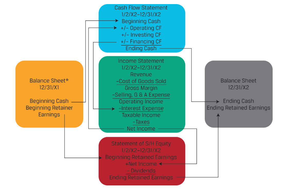
Equity Investments
1. Market Org and Structure
Financial system:
Purpose: (1) saving (2) borrowing money to use now (3) raise equity capital (4) manage risk (5) exchange asset for immediate [spot] / future [option] delivery (6) trade on info
Function: (1) achieve Purpose (2) discover ROR equating aggregate saving / borrowing (3) allocate capital to most productive use
Equilibrium interest rate at Supply & Demand of Money
Traditional VS Alt investment:
Traditional: D&E, Equity swaps (Exchange of fixed cash pay that depend on stock / index return)
Alt Inv: hedge fund, PE, commodities, real estate security, securitized D, OL, machinery, collectibles, precious gems
Products: Commodities (carbon credits), Equity (warrant)
Securities: Fixed Income (Bond, note, bill, Certificate of Deposit COD, Commercial Paper CP, Repo, loan agreement, mortgage) Pooled Inv (ETF = Net Asset Value, in-kind payment - portfolio, among Authorized Participants AP, created by financial intermediaries Ex. S&P)
Real assets: Held by Operating Comp (Real estate developer, manufacturers, loggers), created by financial intermediary (REIT, Master Limited Partnership MLP) Ex. lumber stands
Contracts: Forward (customizable. counterparty / liquidity risk, no cash outlay),
Futures: Clearing house (1) Requires initial margin posted when entering contract (2) Settles margin on daily basis: Deducts / Adds from margin if loss / profit (3) if drop below maintenance margin, participant replenishes account. If not, broker trades to offset position
Financial intermediaries: Ex. commercial, mortgage, IB, credit unions, credit card companies, brokers (fill orders), exchanges (regulated dealers), dealers (broker using own money, provide liquidity), arbitrageur, clearinghouses, depositories (raise fund from depositor, lend), mutual / hedge funds, insurance comp, Alternative Trading Systems [(ATS) = electronic communications networks (ECN) = multilateral trading facilities (MTFs), usually dark pools (no display of orders clients send): trading venues w no regulatory authority]
++ Derivative: 2. Forward Commitment and Contingent Claim Features and Instruments: Option section
* (Financial) Leverage: Use of D in capital structure.
Option Leverage:
Trader’s Equity + Borrowed = Total Purchase
Trader’s Equity: Portion of security price buyer must supply
Borrowed = Margin Loan = Loan traders borrow to purchase security w Call Money Rate (Int, low bc securitized)
Actual Equity Investment requires Purchase /Sales Commission, actual loan requires Call Money Rate
Definitions:
IMR = Initial Margin Requirement = MR on 1st day of transaction, any day additional margin funds must be deposited = Min E% of total purchase price purchase, set by gov / exchange / clearinghouse
MMR = Maintenance Margin Requirement = MR for all other. If E falls below Maintenance MR, buyer receives Margin Call (Request for additional E)
* Max Leverage Ratio = 1/IMR
IMR 40% means 40% is initially invested in equity
* Margin Call Price = Initial Purchase Price × 1 - IMR1 - MMR, subsequent P
* MMR = Equity per sharePrice per share = Initial E p share + Margin Call P - Current Stock PMargin Call P
* Remaining Equity
= Initial Investment (Outflow) + Purchase and Sales Commission Paid (Outflow) + Trading Gain / Loss + Margin Int Paid (Outflow) + Div Received = Remaining Equity OR
= Proceeds on Sale + Payoff Loan (Outflow) + Margin Int Paid (Outflow) + Div Received + Sales Commission Paid (Outflow)
** First Initial Inv includes Commission**
Clearing instruction: How to arrange final settlement
Market regulation: FInancial regulators act to level playing field for market participants, define minimum standards of competence of agents, and require that regulated firms maintain minimum levels of capital
Pim & Secondary Markets:
Financial Systems:
Allocationally efficient: allocate capital to most productive / valuable
Informationally efficient: asset P reflect all avail info
Operationally efficient: low trade arranging costs
Market regulation objectives: control fraud / agency problems, promote fairness, set mutually beneficial standards, prevent undercapitalized financial firms from exploiting investors by making risky investments, ensure LT liab are funded
2. Security Market Indexes
Security Market Index (SMI)
Definition: Proxies for security market, market segment, asset class in asset allocation models. Calculated w constituent securities (indiv securities within index). There are 2 versions of the same index: (TRI > PRI in LT)
Purpose: (1) gauges of market sentiment (2) proxies for measuring / modeling returns, systematic risk, risk-adjusted performance (3) proxies for asset classes in asset allocation models (4) benchmarks for actively managed portfolios [Irrelevant to passive investors] (5) model portfolios for investment products ex. index funds, ETFs
SMI Construction:
Target market, Security selection (investment universe)
Index weighting of securities
Index mngmnt:
Rebalance: adjust weight to maintain consistency with the index’s weighting method
Reconstitution: Rebalance + security. Dramatically affects P of current / prospective constituents
** Calculation:
Value of Price Index
= VPRI = i=1NniPiD
Divisor chosen at inception (usually 1,000)
* Before split of Period 1 must maintain same VPRI by finding the new divisor
Ex.
P before split Period 1: X 10, Y 20, Z 60
P after split Period 2: X 12, Y 19, Z 22
> Period 1:
VPRI = 30 = (10 + 20 + 60) /3
Find adjusted divisor of Period 1: 30 = (10 + 20 + 20) / X
X = 1.67
> Period 2:
VPRI = 31.7 = (12 + 19 + 22) / 1.67
Price Return Index (PRI): Only reflects P change.
Total Return Index (TRI): Reflects revinvestment (div, int)
Multiple Period (Same for PRI, TRI):
VTRIT = VTRI 0(1 + TRI 1)(1 + TRI 2)…(1 + TRIT)
** Weighting Measures
Price weighting: wiP= Pii=1NPi
PRI = ∆%(total index) [총]
Weights arbitrarily determined by market prices
No need for share number
Needs rebalancing only after split, with adjustment to divisor
Equal weighting: wiE= 1N
PRI = (∑∆% Each Security) / n [각각]
Weights assigned by index provider
No need for share number
** requires an adjustment to the divisor after a stock split
Needs 多 rebalancing for equal weighting (P change keeps changing weight), Securities w largest fraction underrepresented / smallest fraction overrepresented.
Market capitalization / Value weighting: wiM= QiPij=1NQjPj
Float adjusted market capitalization weighting: wiM= fiQiPij=1NfjQjPj
Div not included in Index
Constituent securities held in proportion to their value in the target market
Momentum bias: ex. overweighting stocks rising in price
Fundamental weighting: wiF= Fij=1NFj
Weight based on earnings etc
Value tilt: fundamentally weighted index has ratios of BV, earnings, dividends, to market value that are higher than its market-capitalization-weighted counterpart
Contrarian effect: Opposite of momentum: Shift away from stocks rising in price
** If Equal-weighted index price > market-cap-weighted index, comprised of the same securities : Outperformance of small-market-cap due to Contrarian Effect
Equity Indexes:
Broad market index (BMI): 90% of E market
Multi-market index (MMI): Dif country / region in economic / geographics
Sector indexes (SI): economic sectors (consumer goods, healthcare). ∑ SI = BMI. (1) Provides if portfolio manager is more successful bc of stock selection / sector allocation (2) Serves as model portfolio for sector specific ETF
Style indexes:
Fixed Income Indexes:
Issues: (1) large, less regulated (2) dealer market, illiquid
Classification types: issuer, financing, currency of payment, maturity, credit qual, absence / presence of inflation protection
Category: Broad market / market sector / style / economic sector / specialized Index
Alt investments:
Commodity index: Same commodities can have dif weighting methods. Reflects commodities’ futures price and roll yield
REIT index: Illiquid, calculated continuously. Include Appraisal, Repeat sales, REIT Index
Hedge fund indexes: (1) Values determined by (voluntary cooperation of) constituents rather than index providers (2) Biased upward: survivorship bias as reporting is not mandatory
3. Market Efficiency
Efficient markets reflect (Intrinsic / Fundamental Value) prices quickly, only passive investments work, only P only reacts to unexpected changes.
Factors that affect market efficiency: Market participants, informational availability & financial disclosure, limits to trading (allow shortselling!), transaction cost (exploit inefficiencies / arbitrages) and info acquisition cost
Forms of Market Efficiency:
Inefficient / weak form (Reflects Market): No active trading / abnormal return (passive > active mngmnt). Market adjusts slowly to unexpected news, Market val & Intrinsic val discrepancies
Semi-strong-form (Reflects Market + Public): No active trading / abnormal returns (passive > active mngmnt)
Strong-form (Reflects Market + Public + Private)
Technical analyst examining historical data to look for patterns / exploit trading rules) assumes Weak form inefficient, Fundamental analyst assumes Semi-strong inefficient (find intrinsic val w public info to see if mispriced)
Market pricing anomalies: Inefficiencies that are consistent (not due to data mining / snooping)
Time-series: Momentum / overreaction (depending on loss-aversion = nonsymmetrical compared to risk aversion) anomalies, Calendar anomalies: [Small firm / Turn of the year / January effect (returns higher to reduce tax liability / window dressing), Day-of-the week effect (Monday worst return), Weekend effect (weekends worse returns), Turn-of-the-month effect (End / beg of month high returns), Holiday effect (before holiday high return)]
Cross-sectional: Contradicts semi-strong market efficiency. Ex. Book to market ratios, P/E ratio effect, Value Line enigma
Size effect: small-cap comp outperforming large cap comp on risk adjusted basis
Value effect: Value stocks (stocks with low P/E and Market to Book ratio, high div yield) outperform growth stocks
Others: Ex. Distressed securities effect, Stock splits, Super Bowl, Earning surprise
Closed-end fund discount: traded at discounted prices of NAV, not NAV (bc mngmnt fee, tax burdens from unrealized capital gains, liquidity)
IPO: underpriced as underwriters tend to price them
* Net Asset Value = total market value of the fund’s security holdings less any liabilities
4. Equity Securities
Basics:
Statutory voting: 1 share = 1 vote, Cumulative voting: accumulate & vote all shares into 1 candidate
Div on Pref Share (PS): Cumulative, Non-cumulative (if not given, forfeited), participating (std div + incentive div), non-participating
PE investments: no secondary market, regulatory costs are cheaper. Types include VC, Leveraged / Management Buy Out LBO/ MBO (have undervalued assets, high CF, to restructure and make public again), Private investment in PE (PIPE, public comp selling some ownership to investor in exchange of quick capital)
Non-domestic Equity Securities: Foreign restrictions exist to limit foreign investor control on domestic comp, provide opportunities to domestic investors, reduce capital flow volatility in/out of E market. However, emerging markets have benefited from foreign investment as there is less concern with capital constraints, lack of liquidity in the domestic market, cheaper financing cost, higher transparency / reporting quality. Investing types include:
Direct investing: Pay in foreign currency, investment process must be familiarized, less transparent, more volatile
Depository Receipts (DR): Trades like ordinary share on local exchange but represents interest in foreign comp. DR is subject to company fundamentals, market conditions, analysts’ recommendations, exchange rate movements. Depository receipt created when foreign comp E is deposited in depository bank
(custodian / registar: div pay, stock split, transfer agent). Depository issues receipts representing deposited.
Risk and Return of Equity Securities:
Comp Value:
mngmnt’s goal: Maximize Book Value (= SH equity on BS = total A - L, impactable, increase when NI is retained) of comp & Market Value of E (not impactable, depends on impalpable criterias like expectations)
ROE using BV, Price/Market-to-book ratio
Company and Industry Analysis Framework
5. Industry and Comp Analysis ~ 6. Industry and Competitive Analysis ~ 7. Company Analysis: Forecasting
(1) Industry and Comp Analysis
Research Report includes
Front Matter: Issuer name / security identifier, Analyst rec / target buy or sell P, Disclosure / disclaimer
Recommendation: Analyst rec, Summary of key reasons
Comp Description: Biz model / strategy, Explanatory chart / figure
Industry Overview & Competitive Positioning: Industry size / growth / key driver / market share trend / profitability - historical and outlook, Competitive analysis - Porter’s Five Forces (relative profit potential of comp), Analysis or external industry influences - political / econ / societal / tech / legal / environmental (PESTLE: industry themes), Evaluation of comp’s position / strategy in industry
Financial Analysis: Evaluation of key drivers of rev / cost / profitability / CF / issuer’s use & source of capital, Forecast of key drivers / supporting discussion, Historical / forecasted FS
Valuation: Estimates of comp / security value w target P, Relative / present value approach, Discussion of key inputs / scenario / sensitivity analysis
ESG Considerations: Eval of ESG / risk, Ownership structure / mngmng composition, Execution compensation
Risk: Eval of material down/upside risk and discussion of how they are considered in financial analysis
Basics:
(2) Industry and Competitive Analysis
Classification by country: Ex. country where issuer is incorporated, country of primary listing of its E securities, location of its headquarters, market perception
Performance of comp w cyclical demand is most variable / dependent on econ conditions
Industry growth
Cyclical & mature: crude oil, natural gas, freight transportation
Cyclical & growth: semiconductors, fintech, digital ad
Defensive & mature: utilities, beverage, pharmaceutical
Defensive & growth: biotech, software, game
Profitability measures: Time series of ROIC (public comp), assuming public / private competitors are similar
Lower industry concentration w small competitors in market has high degree of competitive intensity unless the industry is service-oriented, is local in nature, or has high product differentiation
Innovator’s dilemma: firm can (1) investin disruptive innov, declining existing biz but not losing market share or (2) ignore innov and lose market share while continuing strong profit for existing.
(3) Company Analysis: Forecasting
Forecasting
Objects: Drivers of FS line, Individual FS line, Summary measures, Ad hoc objects. (regularly reported)
Aapproach for FS objects: Historical results / Base rate & convergence, Management guidance (more accurate forecasts for CAPEX), Analyst's discretionary forecast (econ forecasts, cyclical, undergoing fundamental change)
Rev:
Top-down objects: (Comp) Growth relative to (Nominal) GDP growth, (Comp) Market growth / share
Bottom-up (aggregated to total rev): Volume & av selling price, Product-line / segment revenue, Capacity-based measure, return / yield based measure
COGS: Forecast as % of sales (Gross margin): crosscheck good, not comparable w dif biz model
Capital investment: Maintenance CAPEX forecast depends on hist dep / amort. Growth CAPEX tied to mngmnt expansion plan / rev growth. Check hist comp practice, mngmnt’s financial strategy, capital req. If no mngmnt guidance or pattern, check PPE capacity
* Variable Cost estimate = %∆ (Cost of revenue + Operating expenses)/%∆ revenue
8. Equity Valuation
Equity valuation tries to find intrinsic / fundamental value of security. (* No holding period consideration) Models to find it includes:
1. PV / Discounted CF Model:
V0 = PV of future expected benefits
Div discount model (DDM):
Use Calc
Expected Cash / Div to be distributed to SH, cash including Cash div, Share repurchase / buyback
Needs prediction of timing / amount of 1st div & other div, div growth thereafter
Buyback can be due to (1) comp believes shares are undervalued / want to support share price (2) flexibility in amount / timing of distributing cash to SH (3) tax efficiency [tax rate on div > tax rate on capital gain] (4) ability to absorb increases in outstanding shares bc of exercise of employee stock option
Cash div payout
Declaration day: Comp issues statement declaring div
Ex-dividend date: 1st day share trades w out div. Price drops amount of foregone div on this day as buyers on this date do not receive div anymore
Holder of record date: Day where SH listed on comp’s book has ownership of shares
* Ex-div date ~ Holder of record date = 2 days, linked to trade settlement cycle
Payment date: Day div is transferred
Irrelevant to valuation: Stock div / bond issues of share, Reverse / stock split
Terminal stock value = Expected value of share at end of inv horizon / selling price
Free CF to Equity (FCFE) model:
V0 = t=1∞FCFE(1+r)t
Div paying capacity. CF avail to be distributed to SH after meeting CAPEX, WC needs
Preferred method, can also use for non-dividend-paying stock
FCFE: Measure of CF generated in period avail for distribution to common SH
= CFO + Net Borrowing – FCInv
CFO = NI + NCC - WCInv [In Appendix below]
Required ROR i = Current expected risk - Rf + βi (Market Risk Prem)
In other words, Cost of Equity = re = E(Ri) = RF + βi [E(RM) - RF]
* Perpetual Preferred Stock Valuation
* Constant / Gordon Growth DDM:
V0 = D0(1+g)r-g = D1r-g
* Two-stage: growth → mature stage
* Multi-stage DDM:
V0 = t=1nD0(1+gs)t(1+r)t + Vn(1+r)n , where Vn = Dn+1r-gL , Dn+1 = D0 (1+gs)(1+gL)
Growth comp
CF0 = 0, Final CF = Vt + Dt (1+gs)t and find NPV
Selling included at last year t
Find CF for only until 1 year before perpetuity starts
* Time Value of Money: PVt = i=1nDt (1+gs)i(1+r)i + E(St+n)(1+r)n where E(St+n) = Dt+n+1 (r-gl)
2. Multiplier / Market Multiple Model:
V0 = Share P or Enterprise Value (EV) multiple on forward / trailing basis. For similar comps
Share Price Multiples (= screening mechanism):
Ex. P/B, P/S, P/CF
Higher = Overvalued
Advantage:
Allow relative comparison cross-sectional / time series within sector
Can be stated in forward basis (forecasted EPS) or trailing basis (EPS of most recent yr)
Using fundamental variable (rev, earnings, CF, BV) takes into account future expectations
Disadvantage: stock may be undervalued compared w benchmark, overvalued when compared w intrinsic val estimation. Cyclical comp influenced by current econ conditions
** Justified Forward PE = P0E1 = D1 / E1r-g = pr-g, p = Div Payout Ratio, E = Earning
Enterprise Value EV Multiples (= cost of takeover):
Ex. (EV) / (EBITDA or Total Rev):
EV = Market Cap + Market Value of Pref Stock + Market Value of Debt - Cash and investments
Higher = Overvalued = investors are willing to higher prem for each EBITDA
Advantage: Useful when comparison different capital structure
Disadvantage: May be hard to get MV of D
3. Asset Based Valuation Model:
V0 = Fair Val or Intrinsic Val of A&L = [MV for A (cash, AR, inv, net fixed asse) - L(AP, Note Payable : no LT debt or equity)] / shares, multiply any Market Value to each section
Advantage: For comps w high CA, CL. For private comps
Disadvantage: MV, fair val hard to estimate for inflationary times. Not for comps w high intangibles, PPE
Fixed Income (FI)
1~5. Features, Types, Issuance, FI for Corp & Gov
Basics:
Bond indenture = legal contract
Source of repayment: Gov (tax, infra), comp (CFO, security / lien / pledge / collateral)
Covenant:
Affirmative: Use of proceeds from bond issue, timely FS, allow bondholders to redeem bond at prem to par if issuer is acquired pari passu, cross-default. No additional cost
Negative: Investment limitation, debt issuance senior to existing, asset disposal. restrictive
Yield Curve: YTM of bonds from same issuer across maturities
FI Types: (1) Bullet bond,
In Bullet Pay, the int would remain as the first picture’s 4.8
FI Contingency Provisions: Clause in legal doc allowing action if event / circumstance occurs. Ex. Option
Call: Right to Buy underlying / Put: Right to Sell underlying
Convertible:
Warrant: Holder has option to call at fixed exercise price until expiration date
Contingent Convertible Bonds (CoCos): Bonds that automatically convert to equity if specific event occurs
Fixed Price Call Provision: Issuer can call back bond at predetermined P in future
Make-whole Call: Issuer can call bond at price (YTM of sovereign bond of similar maturity + spread)
FI Types- Area (A: Domestic)
Foreign bond: Bonds sold in A, dominated by A currency, issued by B
Small emerging markets: usually domestic bond issuance (sovereign + local financial intermediary)
Euro / bearer bonds: Bonds issued in B, dominated by B currency. Registered (clearing system: serial number / name)
Global bonds: Bonds issued in Eurobond market and domestic country simultaneously
Issuance and Trading:
Investment grade: BBB- or higher
FI index is dif from Equity index as (1) single issuer can have multiple FI securities outstanding = larger # of bonds (2) finite maturity / higher frequency of new issuance = monthly rebalancing (3) weighted by market value of debt outstanding (like Market Cap of Equity Value)
FI markets are quote-driven or OTC markets
Debut issuer: Issuer approaching bond market for 1st time involves a transfer from private to public ownership to replace bank loans with bonds
FI Markets for Corporate Issuers
FI Markets for Gov Issuers
Public sector vary, use cash-based accounting, exclude dep of fixed public goods (federal highway)or accrual of unfunded liab (gov pension obligation)
Under Recardian (+MM) equivalence, taxpayers expect gov debt to be offset by higher future taxes thus sovereign gov should be indifferent between collecting taxes today VS raising debt of any maturity based
Sovereign bond is issued thru public auction led by national treasury. Once auction announced, investors can submit competitive (specify acceptable P & #) and non-competitive (accept P determined thru action). All non-competitive bids are accepted and competitive bids are ranked w lowest yield (=highest bond P). Single price auctions have all winning bidders to receive same P, coupon. It results in lower cost of fund, broader distribution. Multi-price auction has dif P for each bidder. It results in narrower distribution of large bids bc investors must accept bonds at their bid price
On-the-run: most recently issued bonds used for benchmark yield analysis
Investors have varying non-economic objectives (Ex. reserve requirement)
General Obligation bonds: Non-sovereign gov authorities issuing to repay from local tax CF
Revenue bonds: Non-sovereign gov authorities issuing for specific project. They have maturities matching the expected life of matching project CF
Supranational issuers target bond investors in major currencies using global bond markets. They are agencies, sponsored and owned by multiple sovereigns
6. FI Bond Valuation ~ 8. Yield & Yield Spread Measures for Fixed / Floating Rate Bonds
Bond Valuation
Market Discount Rate MDR (i/y or r, ROR required by investors given risk of bond) = Required Yield = Require ROR = = YTM (IRR on CF where when future CF discounted at this rate, sum PV = bond P)
PVFull = PVFlat + AI
Relation between Bond P: Greater Δ%P if smaller coupon, rising,
Coupon effect: Low Coupon (PMT) makes greater Δ%P (from MDR change)
Maturity effect: LT bond makes greater Δ%P (from MDR change)
Convexity effect: |MDR %Δ increase| > |MDR %Δ decrease|
Bond P & characteristic (more volatile if MDR falling, coupon smaller, LT = higher risk)
** low coupon rate has more interest rate risk as bond value comes at repayment of face value (end)
Fixed Rate Bond Measures
Basics:
Yield measure usually annualized. If more that 1 yr maturity, annualized + compounded
Effective Annual Rate (EAR) has periodicity / compounding of 1 (right side of pic)
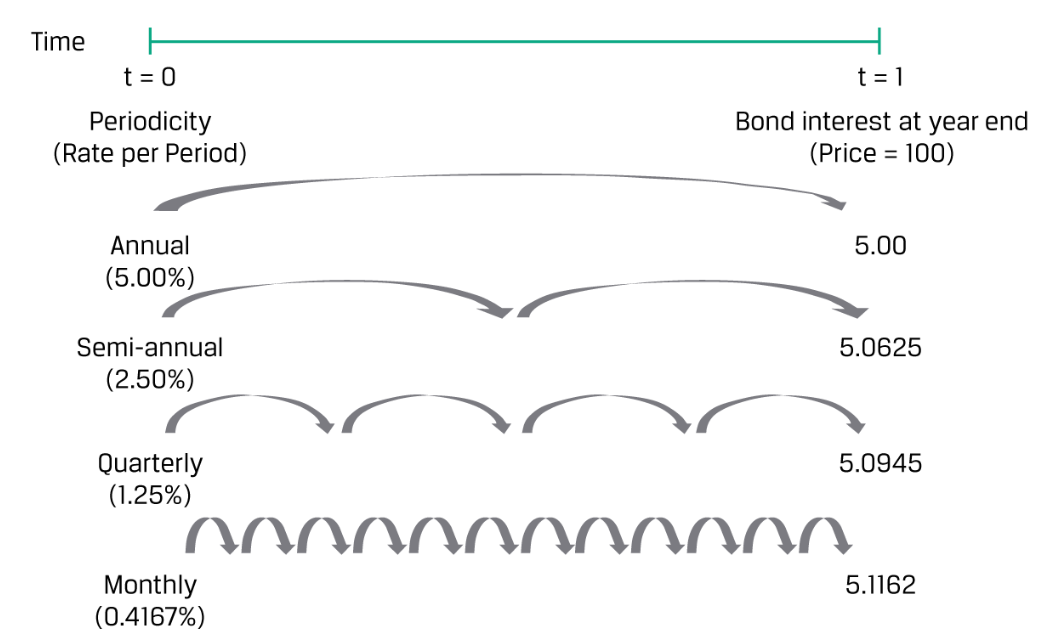
Ex. Q. A bond issued by RTR pays a quarterly coupon of 3.25%, has three years to maturity, and is currently trading at 97.28. The semiannual bond basis yield is closest to:
PV= -97.28, FV= 100, n=12, PMT = 0.8125, CPT I/Y,
Quarterly Yield I/Y=1.055
Quarterly Yield annualized:4.22 = 1.055*4
Annualized quarterly yield → Semiannual bond:
2nd ICONV NOM = 4.22, C/Y = 4, EFF compute:
EFF = 4.287
Change C/Y to 2, CPT NOM = 4.242
Conventions
Current Yield (CY) = Annual coupon / Bond P
Street convention: Yield neglecting holidays, weekends
True yield: Yield including holidays, weekends
Government equivalent yield: Yield restating YTM based on 30/360 to actual/actual
Simple yield: Sum of coupon payments +SL amortized share of the gain / loss, divided by flat price
Spreads:
G-spread: yield spread over gov bond
I-spread: yield spread over standard swap rate w same tenor / currency. Issuers use to determine fixed-rate bonds VS floating-rate alternatives. Investors use to measure of bond credit risk
Z-spread: zero-volatility, constant yield spread over gov / swap curve, showing amount that needs to be added to each benchmark spot rate to make PV of bond’s CF equal to price
When accounting for multiple discount rates, calculate individually
Floating Rate Measures
9. Interest Rate’s Term Structure: Spot, Par, Forward Curve
* Bonds may have different YTM due to credit risk, dif currency, liquidity, tax dif, periodicity assumption, and different times to maturity. Maturity Term Structure of Interest Rates are formed thru recent zero coupon bonds & spot rates (YTM of zero coupon rate).
Use of Spot Rates:
Determine Par Rates: YTM or coupon making PV of bond’s CF = par when differing spot rate per yr
Finding Bond Price
Implied Forward Rate or Forward Yield:
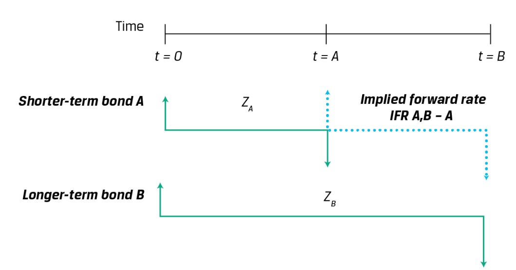
IFR: Breakeven reinvestment rate = Int rate over future period implied by current term structure of int rate. Links ST < zero coupon bond
Convention: 2y5y = 2 years forward into 5 year maturity
First #: length of forward period in years from today (~ in 2 years)
Second #: bond tenor or time to maturity (5Y forward rate ~)
When calculating 2y5y with spots, you are finding 5y’s IFR
(1+ZA)A × (1+IFRA, B-A)B-A = (1+ZB)B
Ex. (1+2yrs spot) (1+IFR)3 =(1+5yr spot)
ZA = Spot Rate
ZB = LT / Total Spot Rate
IFR = Implied Forward Rate
B-A = tenor
Ex. Find PV when Forward rates of 0y1y, 1y1y, 2y1y given to find 3 yr spot rate:
(1+ZA)A × (1+IFRA, B-A)B-A = (1+ZB)B to find Z2 then Z3
(1) Implied rate: Calculate each year’s implied spot rate: 0y1y * 1y1y = (1+Z2)2, 0y1y * 1y1y * 2y1y = (1+Z3)3 , PV = sum pPMT / (each year’s implied rate)n]
(2) Forward rate approach:
Spot, Par, Forward Curve
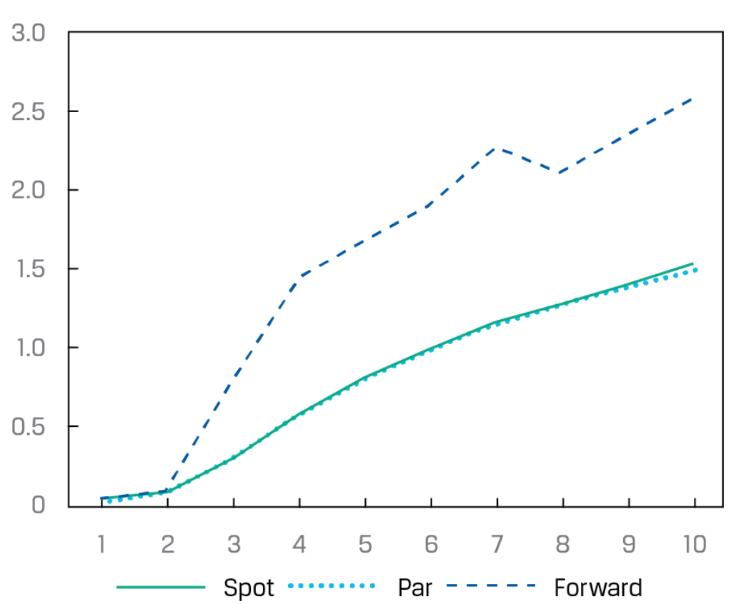
Upward sloping: Par < Spot < Forward
Flat Term Structure: Par = Spot = Forward
Downward sloping / Inverted Structure: Par > Spot > Forward
10. Int Rate Risk & Return ~ 11. Yield-Based Bond Duration Measures & Properties
How does Int Rate change affect coupon payment’s reinvestment & bond P if sold prior to maturity?
Horizon Yield (Realized ROR): Investor’s total ROR on FI over holding period, including reinvested coupon = IRR expressed in annualized rate. Horizon Yield = original YTM if (1) Coupon pay reinvested at same int rate as original YTM (2) Bond is sold at P on constant-yield price trajectory (p on trajectory = carrying value) = no capital gain / loss when sold
r = (FVPV)1T-1
FV = YTM or Future value of reinvested coupon + Sale price in X years (PV usually 100 unless change in interest + sold. If so, recalculated to find PV by n= Total year
YTM = coupon + interest on reinvestment of coupon
Carrying Value
= Purchase Price + Amort Amount of Discount if purchased at P below par value
= Purchase Price - Amort Amount of Prem if purchased at P above par value
Ex.
A buys bond 10 yr 6.2 annual coupon, HTM, YTM = 6.2:
I/Y = 6.2, N = 10, PV = 0, PMT = 6.2
FV of Coupons = 82.493
Redemption Value or Sale Price = 100
r = 0.062 = 82.493 + 100100110 -1
A buys same bond but sells after 4 yrs
I/Y = 6.2, N=4, PV = 0, PMT = 6.2
FV of Coupons = 27.203
Redemption Value or Sale Price = 100
r = 0.062 = 27.203 + 10010014 -1
A buys same bond, int increases to 7.2
I/Y = 7.2, N = 10, PV = 0, PMT = 6.2
FV of Coupons = 86.475
Redemption Value or Sale Price = 100
r = 0.0643 = 86.475+100100110 -1
A buys same bond, int increases to 7.2, sells after 4 yrs
I/Y = 7.2, N=4, PV = 0, PMT = 6.2
FV of Coupons =27.609
Change in int affects bond P
I/Y = 7.2, N=6, FV =100, PMT = 6.2
Redemption Value or Sale Price= PV = 95.263
r = 27.609 + 95.26310014 -1
Notice the power ¼
** Change 100 if bought for discount / prem
As seen above, Fixed Rate Bond’s investment horizon is key to understanding Int Rate Risk & Return. Offsetting types of interest rate risk that affect bond investor is:
Reinvestment risk: Risk is the lower Int Rate. ↓ Rate = ↑ Future val of reinvested coupon payment
Definition- Risk of not matching the bond's yield to maturity (ROR) when reinvesting
Buy&hold investors, LT, higher coupon rate have higher reinvestment risk
** Zero coupon is not exposed to reinvestment risk as there is no CF until maturity
Price risk: Risk is the higher Int Rate. ↑ Rate = ↓ Sale price of bond that matures after horizon date
In other words, if investor wishes to sell bond prior to maturity, sale price will be lower if rates are higher
Sell before maturity, ST have higher price risk
** Macaulay duration (years):
=  =
= 
Definition:
Bond’s sensitivity to int rate change
PV weighted av time / holding period to receipt of CF, which balances Reinvestment risk & Price risk for a 1 time instantaneous parallel shift in yield curve
Relationship:
Lower duration if (Inverse relationship w): Increase in Coupon Rate (c), YTM (r), Fraction for current coupon period that has elapsed (t/T)
Higher duration if (Direct relationship w): Increase in Time to Maturity (T)
** For discount bonds, for a given coupon rate, LT discount bond can have lower duration esp when long remaining number of period, Coupon rate < YTM (discount)
Calculation
Period, Time to Receipt, CF, PV (of CF), Weight (/100), Time to Receipt × Weight
Period & Time to Receipt:
If calculation is done at issuance or on coupon date, they are equal
If not, Time to Receipt = n - (t/T) where t =days since per started
CF: CF or PMT / (1+r)Time to Receipt
** Time to receipt be careful esp if not full number!!)
PV = CF all CF (= PMT) and last as 100+CF, then calculate NPV. 100-NPV = PV
Weight: CF amount / PV: PV is 100 if to par. If not, YTM > Coupon = Discounted Full Price
∑ (Time to Receipt × Weight)
| Dominant Risk | Source of Int Rate Risk |
Investment Horizon > Macaulay Duration | Reinvestment Risk (neg gap) | Falling Int Rate |
Investment Horizon = Macaulay Duration | Same risk |
|
Investment Horizon < Macaulay Duration | Price Risk (pos gap) | Rising Int Risk |
** Annualized Modified Duration (AnnModDur):
= Mac Dur(1+r) = (PV-) - (PV+)2 (∆Yield) PV0 :
Definition: First deriv of bond’s P w respect to yield. Estimates %∆P for given ∆YTM
** Use previous r before change
%ΔPVFull ≈ – AnnModDur × ΔAnnYield
If high ModDur, steep in Price-Yield graph
** Money Duration (MonDur):
= AnnModDur × PVFull
Definition: Estimates ∆P given ∆YTM in currency units (∆Market Val), stated per 100 of par val / actual position size
%ΔPVFull ≈ - MoneyDur × ΔAnnYield
** Price Value of a Basis Point (PVBP):
= (PV-) - (PV+) 2
12. Yield-Based Bond Convexity and Portfolio Properties
Convexity:
Description for curved, non-linear shape of the price/yield relationship of FI instrument
Complimentary risk metric for second-order (=non-linear) effect of Δyield on P for option-free rate bond
13. Curve-Based & Empirical FI Risk Measures
<I can not do this anymore. I will come back to this later>
14. Credit Risk
Credit Risk is the risk for borrower to default. The C’s of Credit Analysis include:
Bottom-up Factors: Covenants, Capacity (ability to repay on time), Capital (Resource avail to reduce debt reliance), Collateral (Asset qual), Character (mngmnt quality)
Top-down Factors: Conditions, Country, Currency
Ex. Corporate CF from (1) Biz op, Inv / financing activity (2) Asset sale, divestiture (subsidiary selling), D/E issuance. Sovereign CF from (1) Tax, tariff, fee (2) Debt issuance, sale of public asset / privatization
Loss Calculation:
EL ($): Expected Loss = LGD × POD ≈ Credit Spread = Probability-weighted amount of loss
LGD ($): Loss Given Default = EE × (1-RR)
POD (%): Probability of Default: Conditional probability of borrower default, assuming no prior default
** If Credit Spread > POD × LGD, fairly compensated for assuming credit risk
Credit Ratings
Credit Migration / Downgrade Risk: Risk where issuer’s creditworthiness deteriorates, migrates lower, making investors believe risk of default is higher
Credit Ratings seeks to assess expected loss
Market pricing of credit risk for distressed bonds focuses on default timing, expected recovery rate
Credit rating outlooks are more aligned with market conditions than credit ratings
Factors impacting Yield: Credit spread risk is the risk of greater expected loss bc change in credit condition. Factors:
Bond Yield (r or I/Y):
Yield Spread:
Liquidity Spread: PV as bid & ask price, finding r then their differences
Credit Spread: r - Benchmark yield - Liquidity spread
Benchmark Yield
15 ~ 16. Credit Analysis for Gov Issuers & Corp Issuers
Sovereign Issuers: Creditworthiness depends on
Qualitative:
Gov institution & policy: Stable, predictable executive, legislative, judicial institutions and policies. Willingness to pay. Rule of law
Fiscal flexibility: Ability to adjust revenue, expenditure. Fiscal discipline. Prudent use of debt
Monetary effectiveness: Policy credibility. Exchange rate regime. Financial system, debt market development
Economic flexibility: Economic diversification. Competitiveness. Adaptability to shocks
External status: Global currency status. Access to external funding. Geopolitical risk
Quantitative:
Fiscal strength:
External stability: Balance of payments,
External debt burden: External Debt Burden (LT External Debt / GDP), External Debt Due (External Debt Due in 12 m / GDP)
Currency reserves: FX reserves to GDP or External Debt
* sovereign gov is creditworthy if domestic currency is a reserve currency (one fully convertible, held by foreign central bank, investors)
Economic growth and stability: Cyclicality,
Economic growth and volatility: Av RGDP growth, Real GDP growth volatility (SD)
Size / income level: econ size (GDP in PPP terms)
Per capita GDP: GDP / Population
Non-sovereign credit depends on issuer: Agencies (quasi-gov), public banks, supranationals, regional governments. In US, municipal issuers (state / local gov) are rated individually and issue:
General Obligation (GO): Unsecured bond backed by general rev of non-sov gov supported by taxing authority to issuer. Used to finance specific project financing
Revenue bonds: Issued to finance specific projects, has higher risk than GO as CF dependent on single source of rev. Analysis similar to corp analysis, w key credit measure of Debt Service Coverage Ratio (rev avail to cover principal, int after op exp)
Corporate issuers depend on:
Qualitative:
Corporate governance: Appropriate use of proceeds, treatment of debtholder / legal, tax, account, covenant compliance
Business model: Demand / rev / margin stability & predictability, Asset quality
Industry & competition: Structure, concentration, competitive forces, LT growth & demand
Business risk: Deviations from expected demand, rev, margin
Quantitative:
Macro (top down) approach: Macro (GDP growth, cyclicality), Industry (Addressable market, market share), Event risk (Scenario analysis, external shock)
Issuer specific (bottom up) approach: BS - Liquidity leverage, profitability. IS - Rev growth, op profit. CFS - Debt service or Int coverage
Creditworthiness ratios: Profitability (EBIT margin), Coverage (EBIT to Int Expense), Leverage [Debt to EBITDA, RCF to Net Debt (Retained CF / {Debt - Cash, MS})]
Seniority ranking: (in priority of claim order)
Secured Trench w direct claim: 1st lien / Mortgage (asset / property pledged) → Senior secured → Junior secured
→ Unsecured Trench w general claim: Senior unsecured → Senior subordinated → Subordinated → Junior subordinated
→ Equity
* In case of default, absorb from equity up
Corp Debt has Rating agencies provide
Issuer credit rating (Corporate Family Rating): Apply to senior unsecured debt, address obligor’s overall creditworthiness
Individual issue rating (Corporate Credit Rating): Specific financial obligation of issuer, takes factors like seniority into account
POD for issuer & issue may be same, but LGD may differ due to seniority, subordination, source of repayment (= notching). Notching is usually done for lower rated seniority
17~19. FI Securitization, ABS & MPS Market Features
Order: Assert transfer from Originator to SPE (Original source of asset → Pooled assets w similar feature → Bank sells to SPE) → SPE issues ABS to investors (SPE → ABS → ABS investors)
SPE & originator signs purchase agreement + prospectus (structure of securitization), trustee safeguards assets
SPE is not affected by the bankruptcy of the seller of the collateral
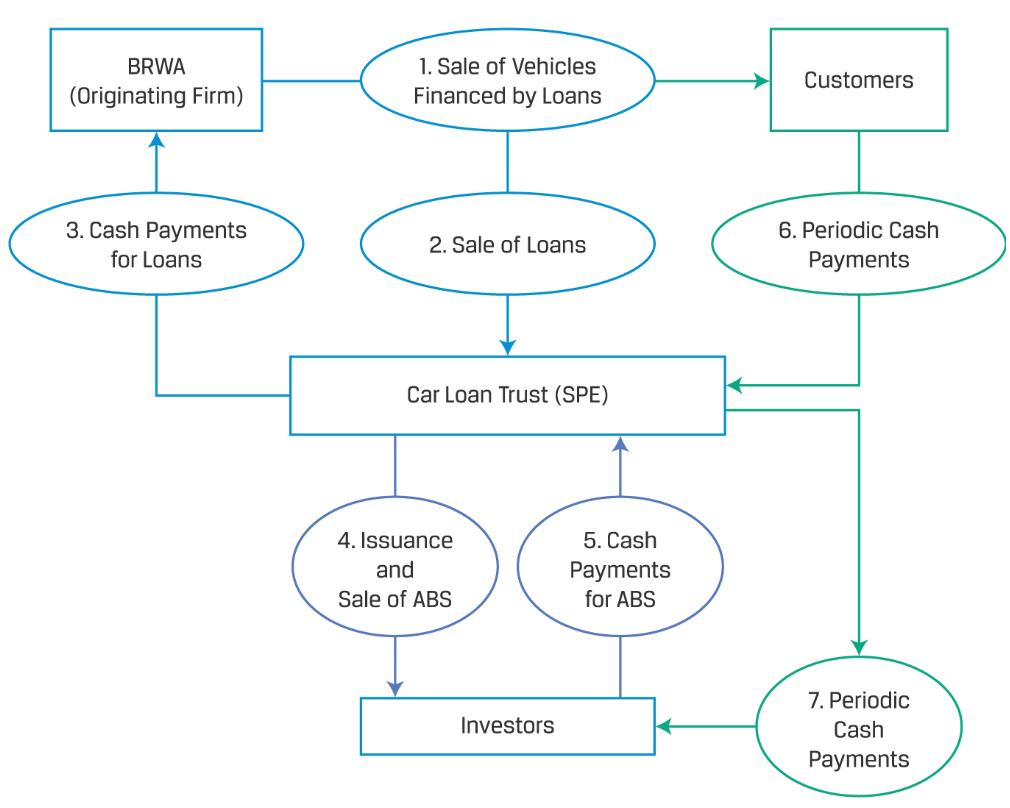
ABS examples:
(1) Covered Bond (CB):
Collateral: Commercial / Residential mortgage, public sector assets. Remains on BS = Not full securitization
Consist of 1 bond per cover pool (unlike ABS)
Dual recourse nature: Ringfenced loans in cover pool, Unencumbered assets on issuing institution
Lower credit risk & yield compared to other ABS due to recourse nature, strict eligibility criteria, dynamic cover pool, redemption regimes in EOD
Investor risk mitigated thru Overcollateralization, Set LTV (Loan to Value), 3rd party monitoring
Ex:
Hard-bullet covered bond: If delayed pay, bond default triggered, payment accelerated
Soft-bullet covered bond: If delayed pay, bond default and accelerated payment delayed until new final maturity date (= 1 yr after maturity date)
Conditional pass-thru covered bond: If delayed pay, convert to pass-thru securities after original maturity date
(2) Collateralized Debt Obligation (CDO): security backed by diversified pool of 1 or more debt obligation. Leveraged transaction, where equity tranche holders use borrowed / issued funds to generate a return above the funding cost. Ex: CBO (Bond), structured finance CDO (other CDO)
CLO (Loan): CF CLO (CF from int, principal redistributed into tranch), MV CLO (MV affects value accruing to tranch), Synthetic CLOs (portfolio of credit default swap for other structured securities).
Manager buys and sells debt obligations to (1) paying off holders of the bond classes (2) generating attractive return for equity tranche and manager
After the ramp-up period but before underlying collateral pool loans mature, collateral manager can replace loans in portfolio as long as new assets meet portfolio selection criteria
Recourse limited to collateral pool
Investors in equity tranches take on equity-like risks with potential to earn returns comparable to equities. These residual tranche investors play a key role in whether a CLO is viable or not. The CLO structure has to offer competitive returns for this tranche. Facing these risk/return possibilities puts them in the position of the marginal, price-setting investors
(3) Mortgage Backed Securities (MBS):
** Foreclosure: Allows lender to take possession and sell property to recover funds to satisfy outstanding debt
Considerations:
LTV: ↓ 🙂= ↑ borrower’s equity, ↓default possibility
DTI (Debt to Income ratio): monthly debt payments / monthly pre-tax, gross income
Prime loan = low LTV & DTI, Subprime loan = high …
To calculate securities value, find Prepayment Risk = (Contraction + Extension risk)
Contraction risk: Risk that borrower repays principal / proportion in shorter time period, reducing future payment investor receives. For investors, investors must reinvest the proceeds at lower interest rates, and prepayment option reduces potential price appreciation for bond
Extension risk: Risk that borrower repays principal / proportion in longer time period. For investors, higher int rate reduces value of CF investors receive. Payments investors receive will be discounted at a higher interest rate, and the extension stretches out the payments the investors receive
Time Tranching aims to mitigate prepayment risk
RMBS:
Collateral: Many Residential mortgage, Mortgage as Pass-thru Securities
Contingencies: Prepayment option, recourse loan (lender can ask borrower for remaining loan if unrecoverable w house itself), non-recourse loan
Types:
Agency RMBS:
Non-agency RMBS: Issued by private entities, not guaranteed
Mortgage Pass-thru Security: pooled mortgages w CF as monthly payment of principal, int, prepayments. Mortgage is securitized. A (WAC - weighted average coupon rate from pool) - B (Pass through rate) = service fee for SPE
WAC = ∑[i × CB / (∑CB)]
CB = Current Balance, OR Principal Value
Pool removed from BS, transferred to SPE. SPE issues securities backed by pooled asset
CMO (Mortgage): securitizes Mortgage as Pass-thru Securities. Tranching can redistribute the prepayment risk across the different tranches. Ex. Sequential Pay CMO (time tranching),
Z tranche / accretion or accrual bond: No int until pre-set date w both principal & accrued int payment start. LT and last tranche. Benefits other tranches as it frees up CF so other tranches can distribute. No reinvestment risk
Principal-Only (PO) securities: Only principal repayments (til face value) paid. Sensitive to prepayment & int rate. When int falls or prepayment accelerates, PO value increases
Interest-Only (IO) securities: Only int payments. Usually hedged
Floating-Rate tranch: linked to index / ref rate
Residual tranche: any remaining CF after all obligation. For LT institutional investors / hedge funds. Banks avoid as it bc capital requirements
Planned Amortization Class (PAC): Fixed CF, any prepayment risk absorbed by support tranche
CMBS
Collateral: Few Commercial mortgage
Structure:
Balloon loans, not fully amortizing (= down pay)
Call Protection: Protection against early prepayment. Sequential-pay tranche allows lower level tranches to be prepaid only if seniors are retired. Principal losses are always borne by the junior tranches first. Steps: Prepayment lockout (prepay not allowed) → Prepayment w penalty → Defeasance (Borrower has to buy gov securities portfolio fully replicating remaining scheduled principal + int’s CF, including balloon loan balance. Cost to assemble afforded by issuer)
Indicators for potential credit performance: LTV,
Balloon risk: Risk borrower fails to make balloon pay at maturity, is in default. Lender has to extend loan to “workout period” and modify original terms. Type of extension risk
(4) Non-MBS:
Collateral: Credit card receivables (non-amortizing), Solar lease / loan payment
Lockout / revolving period: Period of no prepayment risk, and principal repaid is reinvested to acquire additional loan w principal = principal repaid. After lockout, principal start to repay
Ex. collateralized Debt / Loan / Bond Obligation, CDO Squared
Credit Card Receivables ABS: Generates additional fee income
Solar ABS: green loans collateralized by debt (mortgages, loans, receivables) that can be further collateralized by a lien pledged on the installed systems, on the property itself, or both. This would combine multiple liens to mitigate default risk
Credit Enhancement for ABS Credit Risks
Internal: overcollateralization, subordination / credit tranching
External: financial guarantee by bank / insurance comp, LOC, cash collateral account
Derivatives
1. Deriv Instrument & Market Features, 2. Forward Commitment & Contingent Claim Features & Instruments
Deriv Basics: Deriv transforms performance of underlying, rather than directly passing thru returns of the underlying to a 3rd party (counterparty). Includes Stand-alone & Embedded deriv (call / put). Types of Firm Commitment include forward / future / swap / contingent claim (option - one party decides when / whether)
Futures (Standard):
Futures contract buyer creates long exposure to underlying by agreeing to purchase underlying later. Seller creates short exposure by agreeing to sell.
Exchange-Trade Deriv (ETD): Market w standard futures, options avail on exchanges set by exchange. Requires Central Clearing Mandate (verification of of transaction execution, payment exchange, participant recording, MTM, collateral delivery upon inception, deposit to minimize counterparty risk). Less trade cost
Ex. Int rate swap clearing process: Deriv trade executed on Swap Execution Facility (SEF), a swap trading platform. → SEF transaction shared w Central Counterparty (CCP) → Novation process: CCP replaces existing trade → CCP becomes counterparty for both financial intermediaries = CCP assumes credit risk → no default risk exposure for both parties
Exchange reserves may impost the below to decrease counterparty default.
Mark to Market (MTM) / Daily Settlement: Each party must deposit Initial Margin (IM) to Futures Margin Account
F0(T) = Today’s open price, F1(T) = Today’s close price
MTM gain / loss = [F1(T) - F0(T)] × n
Margin Balance1 = Margin Balance0 ± Day gain (loss).
If Margin Balance < Initial Cash Margin, Initial Cash Margin - Margin Balance = Margin Call
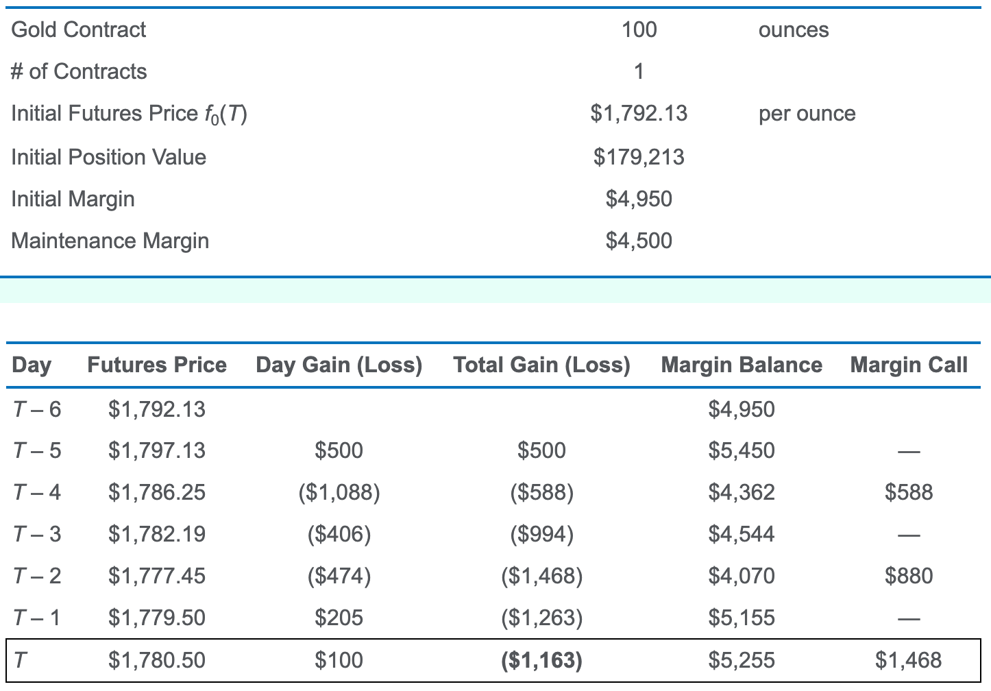
Price Limit: Band relative to previous day’s settlement price within which all trades must occur. Participants require both parties’ agreement to practice outside bands OR impose circuit breaker which pauses indtradahy trading for brief period if a price limit is reached
Forwards (Custom):
OTC: Markets w customizable deriv contracts traded by are driv end users, dealers, financial intermediaries (commercial / investment banks). Less transparent / liquidity
Ex. Long Forward (Forward buyer) Payoff
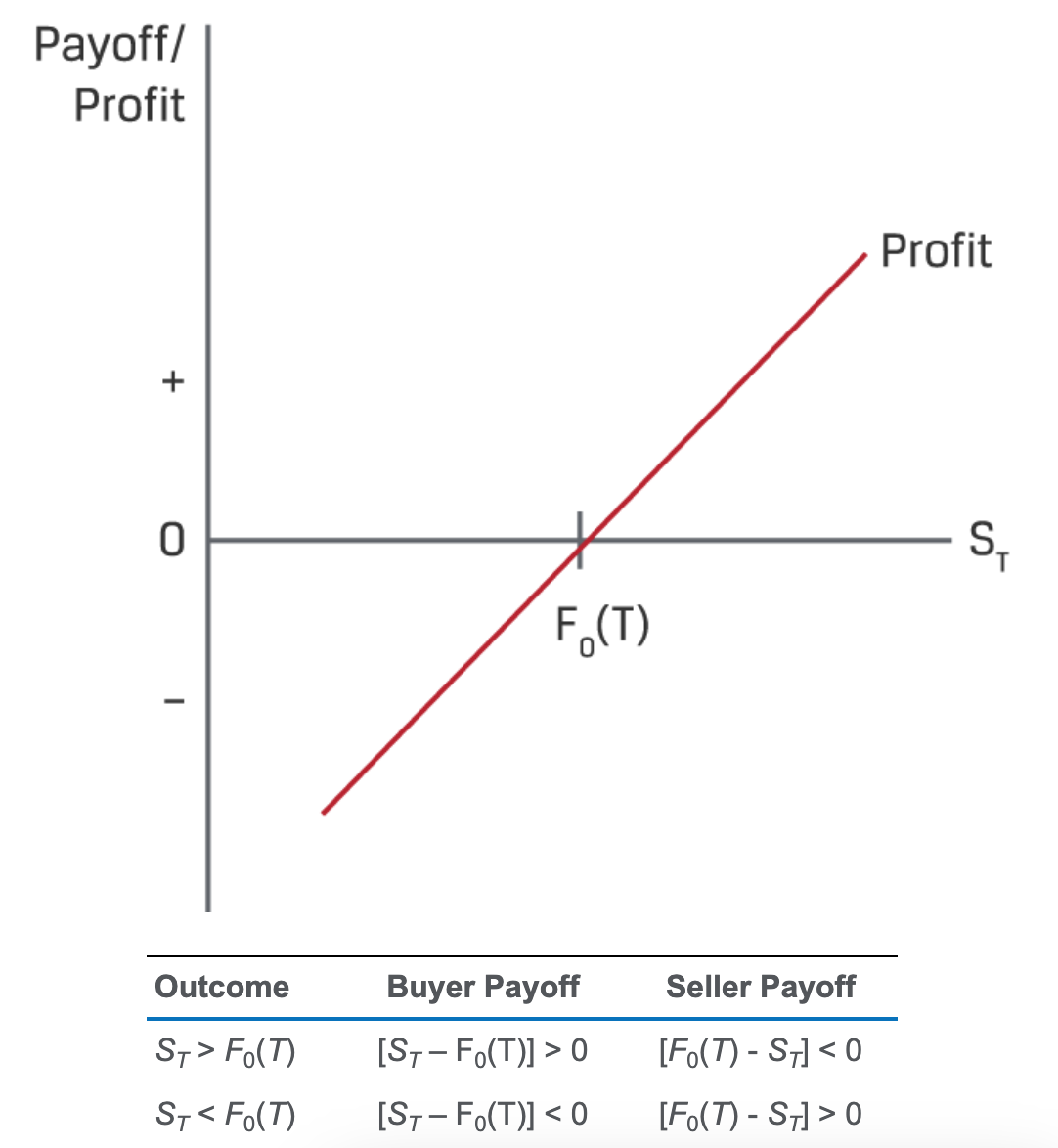
ST = Underlying Price, F0(T) = Forward Price, T = time
Deriv price is a linear function of the underlying, thus firm commitments are linear deriv
At time T, transaction is settled based on difference btw F0(T) and ST from the buyer’s perspective.
Buyer Gain: ST > F0(T)
Credit Deriv
Based on credit underlying = default risk of debt issuer(s)
Credit Default Swap (CDS): Insurance for default. Contingent claim based on Credit Spread like Cash Bond, and Credit Spread depends on POD & LGD. Can manage risk of loss from issuer default separately from cash bond.
Swaps. Counter party: Floating / Fixed Rate Payer
** Options
Option types:
Option positions:
* Ex. Hedgers short if financial risk of instrument positively correlated to exposed risk. Ex. To hedge risk of holding copper, wire manufacturer sells short copper futures. If copper P falls, manufacturer loses copper inventories BUT gains on short position. Long position of inversely related
Option Positions and Underlying Risk |
Type | Position | Exposure to Underlying Risk | Market Expectation |
Call | Long | = Long (upside risk) | Bullish P ↑ |
** Long Call: I hold / buy / own right to buy underlying Risk limited, premium paid (-) Strike Price < Market Spot Price: I want ↑ Underlying Market P so I can practice the buy at strike price lower than market price. If vice versa state, I skip purchase bc i can buy at lower market price outside the option |
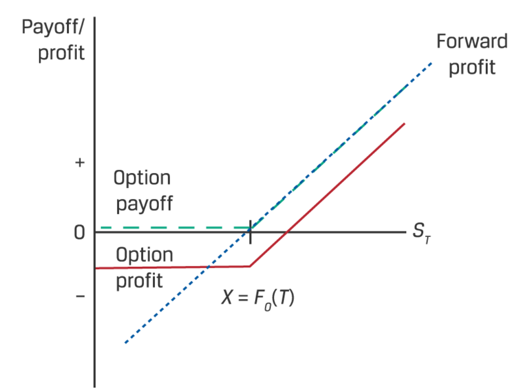
| Original graph: Red Call option value at maturity: cT = max(0, ST - X) Call option buyer’s profit: Π = max(0, ST - X) - c0 Where c0 = Prem |
Short | = Short (downside risk) | Bearish P ↓ |
Short Call: I issued / wrote / sold right to buy underlying from me Risk unlimited, prem received (+) Strike price < Market price: Buyer will exercise, I sell Strike Price > Market Spot price: I want ↓ Underlying Market P, so that buyer passes to exercise, and I receive prem. | 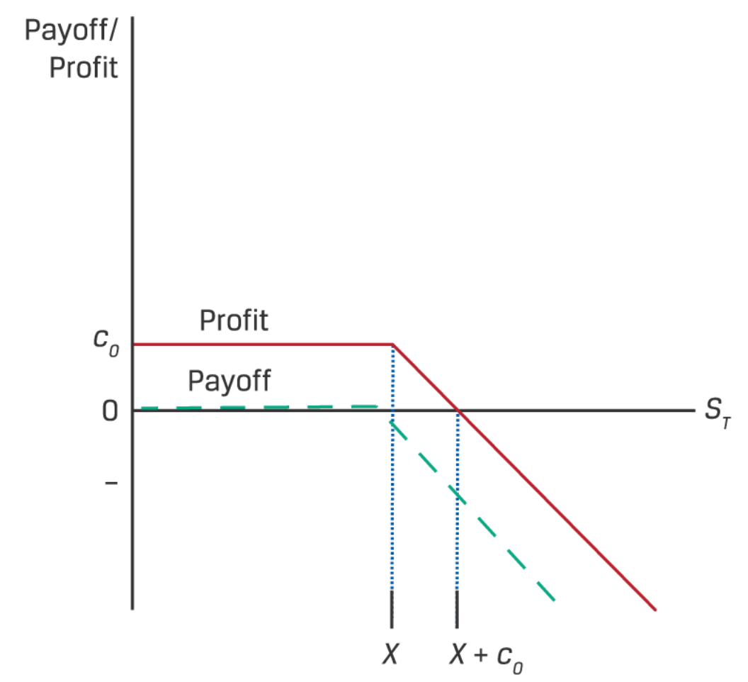
Original graph: Red |
Put | Long | = Short (upside risk) | Bearish P ↓ |
Long Put: I hold / buy / own right to sell underlying Risk limited, prem paid (-) Strike Price > Market Spot Price: I want ↓ Underlying Market P I sell as I can buy at the asset at lower market price and sell at higher strike price at higher price than market price Strike price < Market price, I skip selling as I can sell at higher market price outside the option |
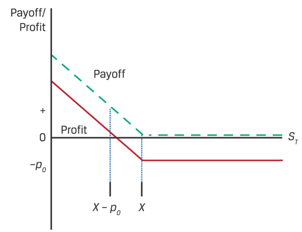
Original graph: Red | long put option payoff: pT =max (0 , X-ST) long put option profit: Π = max (0, X-ST) - p0 |
Short | = Long (downside risk) | Bullish P ↑ |
** Short Put: I issued / wrote / sold right to sell underlying. Risk unlimited, prem received Strike Price < Market Spot Price: I want ↑ Underlying Market P as put option will not be exercised bc put option buyer will not exercise option = sell asset at lower strike price when they can sell at higher market P |
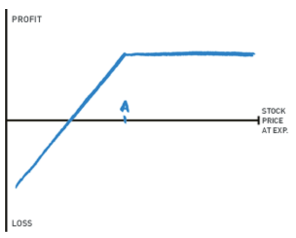 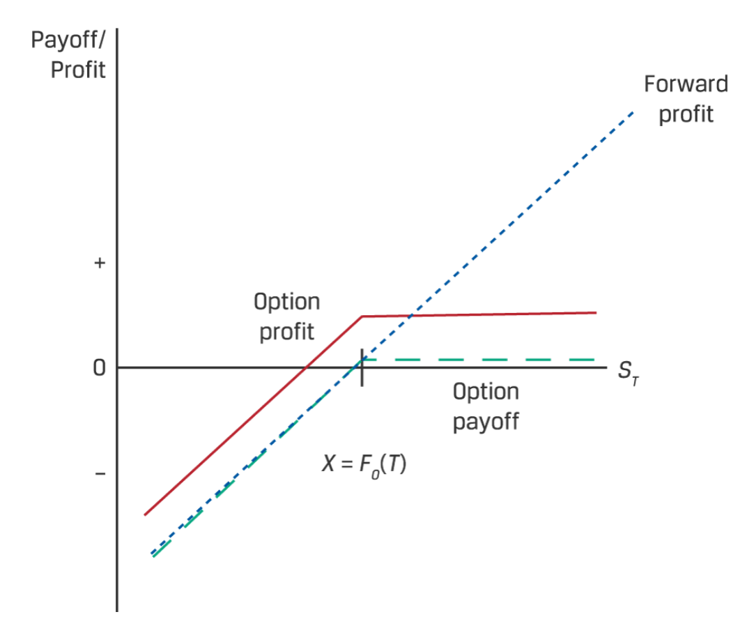
| Shot put option payoff: -pT = -max (0 , X-ST) Short put option profit: Π = -max (0, X-ST) + p0 |
++ Derivative: 2. Forward Commitment and Contingent Claim Features and Instruments: Option section
++ Derivative: 8. Pricing and Valuation of Options
At maturity: Exercise if
Call: (ST − X) > 0
Put: (X − ST) > 0
Any time before maturity (t<T), Exercise Value is:
Call: Max (0, St - X(1+r)-(T-t) )
Put: Max (0, X(1+r)-(T-t) - St)
Assuming F0(T) = X, If ST > PV(X):
St - PV(F0(T)) = Max (0, St - X(1+r)-(T-t) )
Forward Long Commitment at t (Vt(T)) = Call option
Moneyness: Relation btw Option Value & Exercise Price across underlying P
In The Money (ITM):
At the Money (ATM):
Out of Money (OTM):
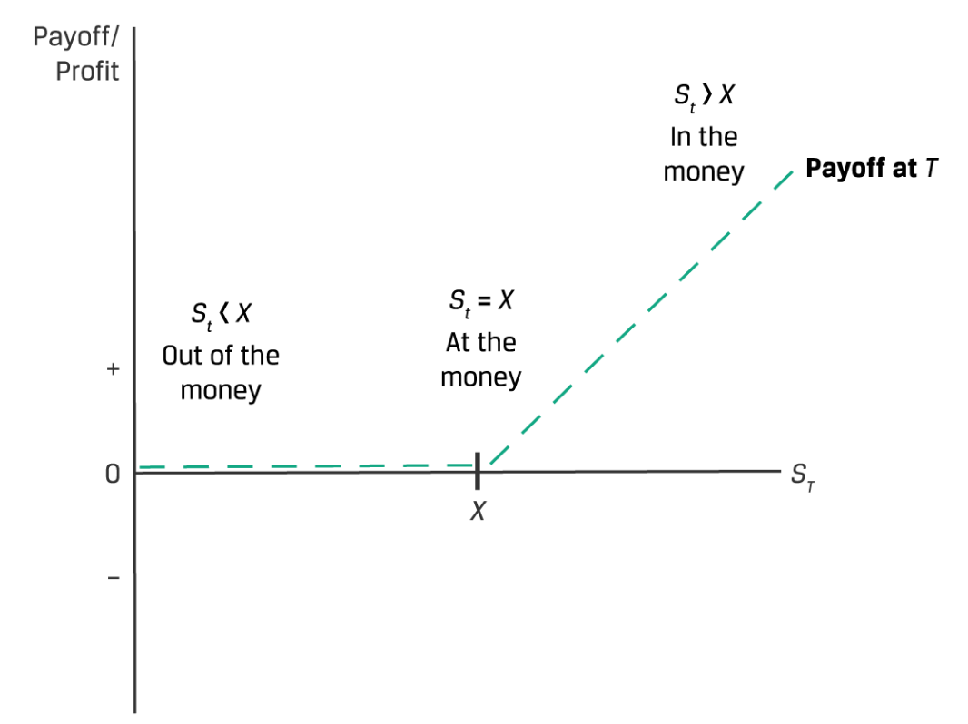
Call Option Time Value: ct - Max(0, St - X(1+r)-(T-t) )
Or ct = Max(0, St - X(1+r)-(T-t) ) + Time Value
Put Option Time Value: pt - Max(0, X(1+r)-(T-t) - St)
Or pt = Max (0, X(1+r)-(T-t) - St) + Time Value
Time Value Decay: time value of an option prem is always positive but declines to zero at maturity. A purchased option declines in value bc of time value defline. A sold option increases in value bc of time value decline
If Exercise Price = Stock Price, Exercise P of both call, put the exercise = 0, only reflect time value
If share price > forward price by more than initial put premium, Loss on forward sale > loss on purchased put at maturity.
3. Derivative Benefits, Risks, and Issuer and Investor Uses
Benefits:
Risk Allocation, Transfer, Mngmnt: Allocate, trade, manage underlying exposure without trading the underlying. Create exposures unavailable in cash markets
Info Discovery: Deliver info regarding expected price in the future, info regarding expected risk of underlying = implied volatility (if goes up, uncertainty of general market goes up)
Operational Advantages: Reduced cash outlay, lower transaction costs versus the underlying, increased liquidity and ability to “short”
Market Efficiency: Less costly to exploit arbitrage opportunities or mispricing
Risks:
Greater Potential for Speculative Use: High degree of implicit leverage increases financial distress
Lack of Transparency: Added portfolio complexity w exposure w out full understanding
Basis risk: Possibility of dif in Expected value of deriv VS underlying. Can arise if deriv references similar P or index
Liquidity risk: Dif in CF timing of deriv VS underlying
Destabilization & systematic Risk: Excessive risk taking, use of leverage contributes to market stress
Counterparty credit risk: Party using futures fail to meet margin call
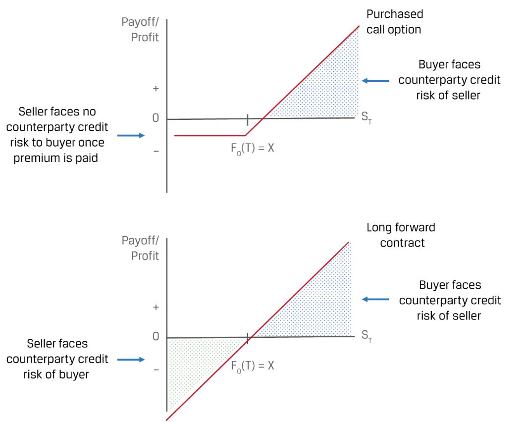 Long Call buyer faces counterparty risk
Users:
Deriv accounting standards require derive purchase / sold marked to market thru IS via Earnings unless embedded in A or L or qualifies for Hedge Accounting. Hedge Accounting allows issuer to offset hedging instruments against hedged transaction / BS items to reduce financial statement volatility. Hedge Accounting Designation types include
CF: Absorbs variable CF of floating rate A or L. Ex. Int rate swap to fixed rate for floating rate debt, FX forward to hedge forecasted sales
Fair Value: Offset fluctuation in Fair Value of A or L. Ex. Int rate swap to floating rate for fixed-rate debt, Commodity future to hedge inventory
Net Investment: Designated as offsetting FX risk of equity of foreign op. Ex. Currency swap or forward
** Upfront prem = Principal at risk + Issue Premium
4. Arbitrage, Replication, Cost of Carry in Pricing Derivatives 5. Pricing & Valuation of Forward Contracts & Underlying w Varying Maturities, 6. Of Futures Contracts, 7. Interest Rates & Other Swaps,
Arbitrage can happen when
2 assets w identical future CF trade at dif price: (S0A = S0B)
Bond A has price of EUR 99 at time t=0: S0A = EUR 99
Bond B has price of EUR 99.15 at time=0: S0B = EUR 99.15
Both bonds have expected future price: S0A = S0B = 100
At time t=0, investor can: Sell Bond B short to receive proceeds of EUR 99.15, purchase Bond A for EUR 99, Realize net cash inflow of EUR 0.15
At time t=1, investor receives EUR 100 for ZBond A, uses this to buy Bond B for EUR 100 to cover short position. Offsetting CF at time T leaves investor w riskless profit of EUR 0.15 price dif between A&B at t=0
Asset w known future P that does not trade at PV of its future price determined using an appropriate discount rate: (S0 = ST(1 + r)–T).
Replication: Deriv’s CF decreased using long / short positions in underlying asset / borrow or lending cash
Cost of carry: Net of costs & benefits related to owning underlying asset for a specific period
Asset Class | Ex | Benefit (i) | Cost (r, c) |
Asset w out CF | Non div paying stock |
| Rf rate |
Equities | Div paying stocks Equity index | Div Div yield | Rf rate |
Foreign Exchange | Sovereign bond (foreign) Market exchange rate |
| Rf - Rd |
Commodities | Soft / hard commodities Commodities indexes | Convenience yield | Rf rate |
Credit | Single ref entity Credit index | Credit spread | Rf rate |
** Convenience Yield = A non-cash benefit of holding physical commodity versus a deriv
Initiation & Maturity is the same, Seller just Vice Versa for all equations
Forward Contract in general
Example for Forward Contract in general:
A agrees to deliver 1,000 shares in 6 months under forward contract. S0 = EUR50, Rf = 5%
Continuous Compounding:
No additional cost:
With cost & benefit:
Currency Market w Continuous Compounding:
No additional cost:
At initiation, Currency w lower Rf rate for forward period trades forward
F0,f/d (T) = S0,f/d e(Rf-Rd)T
During Life, MTM Value of FX forward: Vt(T) = St,f/d - F0,f/d e-(Rf-Rd)(T-t)
↑ Interest rate differential (Rf - Rd) = Price or Foreign currency depreciate on forward basis, Base or Domestic currency to appreciate = MTM Gain
↓ Spot price (S0- < S0) = MTM gain for forward contract seller. This is to satisfy no-arbitrage condition, where S0 at t=0 must equal to PV of forward price discounted at Rf
MTM value for forward seller at settlemenT : F0(T) − ST, seller has a loss if F0(T) < ST
rf > rd = FT,f/d > S0,f/d = Foreign Currency Forward discount = FX Forward Prem
rf < rd = FT,f/d < S0,f/d = Foreign currency forward prem = FX forward Premium Discount
Example for Market w Continuous Compounding w no additional cost
AUD/USD spot P S0,f/d = 1.3335
6M AUD Rf rate = 0.05%
6M USD Rf rate = 0.2%
At time t=0
1) Borrow USD 1,000 at 0.2% USD Rf rate for 6M
2) Purchase AUD 1,333.50 at AUD/USD spot rate S0,f/d
3) Lend AUD 1,333.50 received at 0.05% AUD Rf rate for 6M
At time t=1
4) Receive AUD loan proceeds of AUD 1,333.83 (1,333.50e(0.0005×0.5))
5) Exchange AUD to USD to repay USD at _ST,f/d__
6) Repay USD w interest 1,001 (1,000e0.002×0.5))
If no arbitrage opportunity (Step 4 offset Step 6), ST,f/d = 1,3325 = AUD1,333.83 / USD 1,0001
Interest Rate Forward Contracts
Discount Factor: 1(1+z1)i, P equiv of zero rate = PV of currency unit on future date. Can use TVM
Forward Rates: ** Refer to Fixed Income 9. Interest Rate’s Term Structure: Spot, Par, Forward Curve: Implied Forward Rate
Forward Rate Agreement (FRA): OTC deriv contract w agreement to apply specific int to future period time
IFRA,B-A = Implied Forward Interest Rate
MRRB-A = MRR for B-A period
Initiation: VT(T) =0
Net Payment = (MRRB-A − IFRA,B-A) × Notional Principal × Period
PV of Net Payment: Discounted - FRA settles at the beginning rather than the end of the interest period
fA,B−A = 100 − (100 × MRRA,B−A) = futures price for MRR for B−A periods that begins in A period (MRRA,B−A)

Futures Contract BPV = Notional Principal × 0.01% × Period = ∆P of futures contract given ∆1 bp in yield
Futures Contract - Mark to Market every day, Recognizes Realized MTM, Price fluctuates daily based on market changes, Daily settlement mechanism resets futures MTM = 0, variation margin is exchanged to settle difference and reduce counterparty risk, Cumulative realized MTM gain / loss = comparable forward contract
Forwards Contract - no margin deposit, Recognizes Contract MTM by difference between current spot price St and PV of forward price PV[F0(T)] and is settled at maturity = Counterparty credit risk. Forward Contract Price F0(T) remains fixed until maturity
Swaps: 2 parties exchanging a series of future CF

Pay-Fixed, Receive-Float: MRR > Agreed Fixed rate: MTM Gain (= V of dif btw fixed rate and MRR multiplied by contract notional over int period)
Pay-float, Receive-Fixed, : MRR > Agreed Fixed rate: MTM Loss
Has risk & return profile similar to long fixed-rate bond position
↑Int = Σ PV(Floating payments) > Σ PV(Fixed payments) = will owe more in future floating-rate settlements than it will receive in fixed-rate settlements = MTM loss for the client
Swaps have price and a value: Price is a reference to the fixed-rate payment on the swap, which is constant over time. The value of a swap is zero at initiation but can change over the life of the swap as market interest rates change.
Swap has periodic settlements at end of period (FRA has single settlement in beg of int period)
Swap & forward both hold counterparty risk
Interest rate swap has a constant fixed rate for which PV of fixed versus floating CF exchanges equals zero
Swaps allow issuers to match periodic CF of specific BS liab to transform their int rate exposure profile
Swaps enable investors to actively adjust their interest rate exposure profile w out buying / selling underlying securities
Swaps enable both issuer / investor to avoid admin burden of entering into / managing multiple forward contracts
Par swap rate represents fixed rate at which PV of fixed and future CF equal one another. First find Implied Forward Rate per period using zero rates, discount implied forward rate back to present using zero rate
Periodic settlement value = (MRR – sN) × Notional amount × Period.
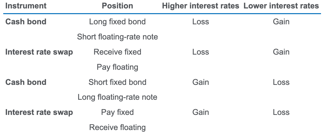
9. Option Replication Using Put-Call Parity
10. Valuing a Derivative Using a One-Period Binomial Model
(I can not do this anymore. I will come back)
Alternative Investments
1. Alternative Investment Features, Methods, Structures
Characteristic: LT, illiquid, larger capital outlay
Ex: PE (mature life cycle stage / firms in decline for leveraged buyouts), Infra (built by gov or Public-Private Partnership PPP thru concession agreement)
Means: Fund investment (just choose, no investment decisions), Co-investment, Direct investment
Fund Investment Structure: 1) pre-commitment of funds prior to investment selection, extended period where fund is not sold, (2) higher mngmnt fees, complex fee structures, (3) less transparency on periodic returns and fund positions
Coinvestment reasons: 1) accelerate investment timing when avail funds, expected inflows are insufficient for specific deal, 2) expand scope of avail new investments, 3) increase diversification of an existing pool of fund investment
Management Fee: Mngmnt fee + performance fee / incentive fee / carried interest based on % of periodic fund return, levied on committed capital (amount LP provides to fund) [VS Funds: fixed % of AUM, based on invested capital]
2. Alternative Investment Performance, Returns
Investment Cycle: Capital Commitment( Investment selection, immediate / delayed commitment of capital = Capital call, Neg returns) → Capital Deployment → Capital Distribution
Shows J-Curve effect
Evaluation be thru (1) IRR or (2) Multiple Of Invested Capital MOIC (3) Leveraged Returns or Cash position rL (4) mark-to-model” valuation
MOIC = Money Multiple:
rL = Simple Leveraged ROR
= r (Vc+Vb) - (Vb+rb) Vc
= r + Vb Vc (r-rb)
r = periodic ROR, rb = borrowed periodic rate, Vc = cash investment, Vb = borrowed fund (borrowed / capital)
Breakeven: rL = r
Mark to Market: Returns are overstated, volatility of returns understated. Accounting valuation through fair value in different levels:
Lvl 1: Accessible quoted P in active market for identical A/. Ex. Exchange-traded public equity securities (observed closing market P)
Lvl 2: Inputs other Level 1 in/directly observable for A/L. Ex. OTC int rate deriv (pricing model using quoted market P)
Lvl 3: No inputs / market activity to measure Fair Val for A/L. Ex. PE, Real estate (CF projection model w avail market participant assumption)
Returns:
GP’s return: Mngmnt Fee + Incentive Fee structure (notation: “rm and p” structure)
Normal return:
RGP = (P1 × rm) + max[0, (P1 – P0) × p]
Net of mngmnt fee:
RGP(Net) = (P1 × rm) + max{0, [P1(1 – rm) – P0] × p}
Net with Hurdle:
RGP(Net with Hurdle) = (P1 × rm) + max{0, [P1(1 – rm) – P0×(1+hurdle)] × p}
High-water Mark (in P2, PHWM = P1 - RGP ):
RGP(High-Water Mark) = (P2 × rm) + max[0, (P2 – PHWM) × p]
Net with High-water Mark
RGP(Net with High-Water Mark) = (P2 × rm) + max[0, {P2(1-rm) - PHWM} × p]
** Fund value = P1 - RGP
Investor’s periodic ROR: ri = (P1 – P0 – RGP)/P0
Redemption fee: Fee charged to discourage redemption, offset transaction cost for remaining investor in fund. Notice period is given in advance for investors to redeem investment. Lockup period is the minimum holding period before investors can withdraw funds. A gate provision limits redemption for a period of time at the discretion of fund manager
Custom Fee Arrangement: include (1) Fees based on liquidity term / asset size (2) Founders shares [incentives for first investors - lower mngmnt fee structure] (3) Either/or fees [major investors can choose lower mngmnt fee or higher incentive fee]
Biases: survivorship / backfill bias
3. Investments in Private Capital: E&D, 4. Real Estate, Infrastructure, 5. Natural Resources , 6. Hedge Funds, 7. Digital Assets
Equity
VC: Pre-seed capital / angel investing → Seed-stage (support development, marketing) financing → Early-stage / start-up (between operation - commercial production for strategic investors) financing → Later-stage / expansion (before IPO) financing, Mezzanine: before IPO, expand
Private Investment in Public Equity (PIPE): Private offering to select investors with fewer disclosures, lower transaction costs allowing issuer to raise capital more quickly and cost effectively
Exit strategies:
Trade sale: Division of private comp sold via direct sale / auction to strategic buyer w intentions for expanding sale / biz scope
🙂immediate / fast / simple cash exit, higher P (prem) from synergy seeking strategic buyers,
🙁potential management opposition, limited buyers, decreased financial appeal w foregone monetization of ownership stakes / options
Public listing:
IPO: for large, fast growing comp, earns market attention
🙂highest potential share prie, likeliest mngmnt approval, PE sponsor’s fame, P appreciation from ongoing ownership stake
🙁high transaction cost, LT, stock market volatility, much disclosure, lockup period freezing capital committed to deal
Direct listing: Security E floated on public market directly w out underwriters to reduce complexity, cost
Special Acquisition Company (SPAC): “blank check” comp existing to acquire unspecified private comp w predetermined period or return capital to investors. earns market attention
🙂extended disclosure time / ability to provide forward guidance to develop investor interest, fixed valuation / lower share P volatility, transaction structure flexibility, high-profile / seasoned sponsors involved
🙁Capital cost dilution, valuation spread (announced / true value from dilution), deal /capital risk of potential redemption, prolonged post-merger stockholder overhand (downward pressure on share P as large blocks are sold in open market) / churn
Recapitalization: via PE maintaining control, increase leverage & pay div out of new capital structure.
Secondary sale: sale of comp to PE
Write-off / liquidation: investment loses value
Debt
Mezzanine debt: Private credit subordinate to senior secured debt, senior to equity
Unitranche debt: Hybrid loan structure (dif tranches of un/secured) in single loan / int rate
Vintage Yr: yr private capital fund makes first investment
Risk & Return: InfraD < Senior real estate D < Senior direct lending < Unitranche D < Debt mezzanine < PE co-investment
Funds seeded during Expansion phase earn excess returns if early-stage comp
Funds seeded during Contraction phase earn excess returns if distressed comp
Real Estate
Debt:
Private - Mortgage / Mezzanine debt, construction loan
Public - MBS / CMBS / CMO, Covered bond, Mortgage REIT / ETF
Equity:
Private - Direct (sole ownership, JV, LP), Indirect (real estate fund, private REIT)
Public - Publicly traded shares, public REIT, UCITS / Mutual fund / ETF
Direct investment: tax benefits (reduce taxable income using non-cash property dep expense, tax deductible int expense)
Indirect investment:
REIT structure eliminates double corporate taxation (usually Corp + personal tax, avoid corp by distributing div) - Trades on exchanges w Master limited partnerships
Strategy (Risk & Return): Senior Debt → Core Real Estate (strat w exposure to well-leased, high-qual comm / res real estate, offered by open-end funds) → Core-plus Real Estate → Value-add Real Estate → Opportunistic Real Estate
Forms: (1) Equity REIT (invest in prop thru partnership) (2) Mortgage REIT (underwrite loan to real estate) (3) Hybrid REIT (invests in both 1, 2)
Infrastructure
CF from contractual payments like (1) Availability payment [payment received to make facility avail] (2) Usage-based payment [toll], (3) Take or Pay arrangement [min purchase price to pre-agreed volume]
Infra has higher recovery rates, lower default rate
Category:
Economic infra: (1) transportation asset (2) info and communication tech (ICT, data center) (3) utility and energy assets
Social infra: ex. healthcare and educational facilities
Investment Stage: (Most risk & return at top)
Greenfield investment: 1st stage of development. Develop new asset to lease / sell / hold & operate. high weighting to capital appreciation
Brownfield investment: 3rd stage of development. Expand existing facilities, use privatization of public assets, sale leaseback of completed greenfield project. ST investment, immediate CF & op history. high weighting to current yield
Secondary-stage investment: investment in existing that needs no development
Natural Resources
| Raw land | Farmland | Timberland |
Return drivers | Land price | Harvest Q, commodity P, land P | Biological growth, harvest Q, lumber P, land P |
Rev source | P appreciation, lease | Crop sale, P appreciation, lease | Tree sale, P appreciation, lease |
Value | location | Location, growth cycle, soil quality | Location, timper quality, timber proudctionphase |
Risk | Alternative use | Weather, biological factors, disease |
|
Owner | Institutional mostly | Individual mostly | Institutional mostly |
Ownership structure | Direct / partnership | Direct / partnership, REIT | Direct, partnership, REIT, TIMO |
* TIMO = timberland investment mngmnt organizations
Commodities:
No CF. Investing usually thru derivatives or funds (commodity trading advisers CTA - various futures)
In case of carrying commodity, F0(T) = S0e(r+c–i)T
Backwardation: Spot > Forward = downward sloping / inverted forward curve, convenience yield > 0, benefit of holding commodity > cost of carry = enhances returns of long-only investors
Low inventories of commodity = incentive for market participants to own physical commodity rather than a derivative contract = incentive drives up spot prices relative to forward prices and lead to S > F = backwardation
Carrying commodity = incurs Cost of Carry (tax, brokerage)
Contango: Spot < Forward = cost of ownership > benefit of convenience yield = lowers returns of long-only investors
Work as hedge against inflation as returns on commodity investing are driven by commodity price changes, and inflation partially reflects these changes
High leverage, perform better during inflationary periods
Hedge Funds
Hedge fund:paid performance based fee, require managers to invest, barely regulated, privately owned, ST
Mutual fund: paid fixed compensation, no own investment, highly regulated
Strategies:
Equity: long/short E (long in undervalued), short bias (short overvalued), market neutral, growth (long), value
Event driven: merger arbitrage (long undervalued / acquired), distressed, special situation, activist
Relative value: convertible bond arbitrage (underlying bond vs embedded call), FI arbitrage (General - sovereign, ABS - mispricings), multi-strategy
Opportunistic: global macro, managed futures (= CTA using momentum of commodities)
Multi-manager: Funds of Funds
Illiquid → Liquid: LP → SMA → Close end funds → Mutual funds → ETF
Risk & Return:
Market beta: systematic, broad market using market index - fund / ETF
Strategy beta: investment strategy of hedge fund
Alpha: manager specific returns from selection of positions
Expose to selection bias (voluntary reporting), survivorship bias
Digital Asset
Distributed Ledger Technology (DLT): tech development offering improvements to deliver financing service
Distributed Ledger: shared database
Consensus protocol: set of rules governing how blocks join the blockchain to resist malicious manipulation thru
Proof of work: determines which specific block to add through computationally costly lottery by miners. Longest blockrain most secured bc computation itself is impossible to manipulate in short time
Proof of stake: requires participants on networks = validators to pledge capital to vouch for block's validity
Forms: Permissionless network: Network fully open to any user on DLT network. All recorded, slower, costlier, decentralized, safer (VS permissioned network)
Appendix
Recognition Models
Fair Value: $ that would be received to sell an asset / paid to transfer a liab in an orderly market transaction
Amortized Cost: ($ A/L is initially recognized) - (principle repayments) ± (amort of discount / premium) - (reduction for impairment)]
Net Realizable Value (NRV): (Estimated selling price in ordinary course of biz) - (Estimated cost to make sale & to get inventory in condition for sale)
Market Value:
[Equity] Value asset can be bought / sold
[Inventory] Current replacement cost of (NRV - Normal Profit Margin ≤ MV ≤ NRV)
Intrinsic / Fundamental Value: Value determined by investor if they completely understand investment. Estimate only.
Net Asset Value = total market value of the fund’s security holdings less any liabilities
FS Ratios |
Activity / Efficiency / asset utilization / operating ratio: day-to-day tasks. Turnovers higher: 🙂 Revenue = Sales |
Days of Inventory on Hand (DOH) | Days in PerInventory Turnover | Av days comp takes to sell inv |
Inventory Turnover | COGSEnd or Av Inv | # of times comp sells inv in yr |
* Analysis: Low DOH, High Inv Turnover: Effective inv mngmnt OR comp doesn’t carry adequate inv / comp written down inv values. Can result in lost sales, production problems for raw materials inv High DOH, Low Inv Turnover: slow-moving inv due to tech obsolescence, change in fashion
|
Days of Sales Outstanding (DSO) | Days in PerReceivables Turnover | Av days comp takes to receive AR Receivable writeoff = ↓ DSO If constant ↑, premature recognition of rev |
Receivables Turnover | RevEnd or Av Inv |
|
Days of Payables Outstanding (DPO) | Days in PerPayables Turnover | Av days comp takes to pay supplier |
Payable Turnover | Purchase or COGSEnd or Av Inv | # of times paid off to supplier in yr |
* Analysis: Low DPO, High Payable Turnover: Not using avail credit facilities OR using early payment discounts High DPO, Low Payable Turnover: Not paying on time OR using lenient supplier terms.
|
WC Turnover | RevAv WC |
|
Fixed Asset Turnover | RevAv Net Fixed A or PPE | Rev from Fixed Asset inv. Low ratio = capital-intensive OR new biz (new asset w less Dep, high Carrying Value) |
Total Asset Turnover (TAT) | RevAv Total A | * In Du Pont |
Liquidity ratio: ST obligations. Low - reliance on CFO OR outside financing |
Current | CACL | WC > 0 → Current Ratio >1 |
Quick / Acid test | Cash + ST MS + ARCL |
|
Cash | Cash + ST MSCL |
|
Defensive interval = Burn rate | Cash + ST MS + ARDaily cash expenditure | Days comp can pay daily cash expenditure w only liquid A, no additional CF. For ventures.
Cash expenditure = ∑ Expense - ∑ Non-cash expense |
Solvency Ratio: LT obligations. Expense = Payment * Total D = Interest bearing S/LT D. No Accrued liab, AP, Lease |
Debt to Equity | Total DTotal E | MV used (not BV) |
Total Debt (to Asset) | Total DTotal A |
|
Debt to Capital | Total DTotal D + Total E |
|
Financial Leverage | Av Total AAv Total E | * In Du Pont |
Debt to EBITDA | Total or Net DEBITDA | Yrs to repay debt based on EBITDA (= Approximate of CFO) |
Interest Coverage | EBITInt Expense | # of times EBIT from op inc covers int payment = times int earned |
Fixed Charge Coverage | EBIT + Lease ExpenseInt Expense + Lease Expense | # of times comp earning covers int & lease payment |
Profitability Ratio: Generate profits from capital invested. Revenue = Sales, EBIT Profit = Op Profit, Earnings Before Tax (EBT) Income = Pretax Income, Profit = Income |
|
Gross Profit Margin (GPM) | Gross ProfitRev | = Rev to cover op & other expense, then generate profit = % of Rev contributed to NI (Int covering Cost of Sales) Gross Profit = Rev - COGS |
Op Profit Margin (OPM) | Op IncRev | Op Inc = Gross Profit - Op Cost * In Du Pont |
EBT Margin | EBT IncRev | EBT = Op Profit - Int Reflects effect on profitability of leverage and other (non-operating) inc & expenses |
Net Profit Margin (NPM), Profit Margin, Return on Sales | NIRev | Net Profit = Rev - All Expense Includes non/recurring components * Du Pont: NPM = Tax burden × Int burden × OPM |
|
Operating ROA | EBITAv Total A |
|
ROA | NIAv Total A | NI = Return to E holders Assets are financed by E holders & creditors, Interest expense (= return to creditors) subtracted in the numerator * Du Pont: ROA = Tax Burden × Int Burden × OPM × TAT |
Adjusted ROA (Pre-int) | NI + Int Expense (1-Tax Rate)Av Total A |
|
Adjusted ROA (Pre-int, Pre-tax) | EBITAv Total A | Return on all asset (liab / D / E) invested in comp |
Return on Invested Capital ROIC | EBIT (1-Tax Rate)Av Total SLT D&E or Av Invested Capital = After Tax OPM × Capital or Asset Turnover | Invested Capital = Op A - Op Liab After Tax Op Profit =After-tax Op ProfitSales Capital or Asset Turnover = SalesAv Invested Capital |
** ROE | NIBeg year Total E or Av Total E | NI avail to common SH earned on E capital (minority / pref / common E) invested after Div Use BV Denominator depends on whether E is volatile (if so, use av) High ROE is not always good Ex. 🙁↑ROE if ↓NI slower rate than SH E or if comp, issues D to repurchase outstanding shares = ↑leverage, risk |
Return on Common Equity | NI - DivAv Comon E |
|
** Du Pont Analysis: ROE = NIAv E = NIEBT × EBTEBIT × EBITRev × RevAv total A × Av total AAv E = Tax Burden × Int Burden × OPM × Total Asset Turnover × Leverage = ROA × Leverage = NetPM × Equity Turnover * Tax burden = 1 - tax rate |
CF Ratios |
Coverage Ratio (IS, CFS) High 🙂 |
Debt Coverage | CFOTotal D | Financial risk and leverage |
Reinvestment | CFOCash Paid for LT A | Ability to acquire asset w CFO |
Debt Payment | CFOCash Paid for LT D | Ability to pay debts w CFO |
Div Payment | CFODiv Paid | Ability to pay div w CFO |
Investing and Financing | CFOCFI & CFF Outflow | Ability to acquire A, pay D, make distribution to owners |
Performance Ratio (CFS) |
CF to Rev | CFONet Rev | Op cash generated / $ of rev |
Cash Return on Asset | CFOAv Total Asset | Op cash generated / $ of A investment |
Cash Return on Equity | CFOAv SH E | Op cash generated / $ of owner investment |
Cash to Income | CFOOp Inc | Cash generating ability of op Can use change in CFO |
CF per share | CFO - Pref Div# of Common Shares Outstanding | CFO on a per-share basis |
Other Ratios |
Valuation ratio, Price / EV Multiple: Quantity of asset / flow evaluating E |
P / Earning | Price per share / EPS = pr-g | p = Div Payout Ratio g = b or (1 - Div Payout Ratio) × ROE p = EPS / Div Payout Ratio * Low P/E and P/B = undervalued |
Price / Book Value | Market Price per share / BVE per share | Investors’ expectations about company’s future investment, CF-generating opportunities Higher 🙂 Compare for similar industries |
Div Payout Ratio | Div / NI = 1 - Earnings Retention Rate (b) | Price to Earning ratio = Div payout ratior-g |
Retention Rate (b) | (NI - Div) / NI = 1 - Div Payout Ratio |
|
Div / Sustainable Growth Rate (g) | b × ROE = (1 - Div Payout Ratio) × ROE |
|
Others |
PPE Asset Age Ratio | Estimated Total Useful Life Hist CostAnnual Dep Expense = Estimated Age of Equipment Accum DepAnnual Dep Expense + Estimated Remaining Life Net PPE Annual Dep Expense | Cost model * Net PPE = PPE – Accum dep (Don’t use the FS’ Net) |
Common Size Analysis: | - IS: Everything / Rev - BS: Everything / Asset - CFS: ① Cash Inflow (Outflow) / Total Inflow (Outflow) ②Everything / Net Rev | IS: Analysis for time-series and cross-sectional comparison (compare comp w each other across time / industry / sector) Identifies strategies BS: Identify strategies & capital structure |
Earnings per Share (EPS) Basics: IFRS and USGAAP require EPS on IS for net P&L, P&L from continuing op Ordinary share / common stock / common share: Equity shares subordinate to all other. Paid last in liquidation, benefit most when comp doing well Diluted EPS = decreased EPS Shares repurchased are (-) 2 for 1 split treated as if happened in beg. Ending WANCSO × 2 to total shares Divs: Pref Div for Non/Convertible Shares are all included (included in converted securities or not ) SH Div is NOT included Common Share issued as Stock Div are NOT weighted, and treated as if issued at beg of yr. Thus add the WHOLE number to WANCSO
Basic EPS: BEPS = NI - Pref DivWANCSO = Income Avail to Common SHWANCSO
Diluted EPS Convertible Preferred Stock DEPS = NI WANCSO + NCSI at Conversion NCSI = New Common Shares that would have been Issued NCSI at Conversion = Convertible Pref Shares × # each Pref Share is convertible into If-converted method: EPS if Convertible Pref Sec were converted at beginning of period. If converted in the beginning, 1) Convertible Pref Securities would no longer be outstanding. Instead, additional Common Stock would be outstanding. Thus WANCSO would be higher than BEPS 2) Comp would have not paid Pref Div. Thus, NI avail to Common SH would be higher than BEPS
If Stock is not convertible, it is left to (-pref div) and left out of WANCSO change
Convertible Bond / Debt DEPS = NI + After Tax Int for Convertible Debt - Pref DIv WANCSO + NCSI at Conversion If-converted method: EPS if Convertible Debt were converted at beginning of period. If converted in the beginning, 1) Debt Securities would no longer be outstanding. Instead, additional Shares of Common Stock would be outstanding 2) Comp would not have paid Interest on the Convertible Debt. Thus, NI avail to Common SH increases by After Tax Int for Convertible Debt
May be dilutive or anti-dilutive NCSI Bond converted = (Total Convertible Bonds / Face Value per Bond)(Common Stocks each Bond is Convertible into)
Convertible Stock Option (Employee, Warrants) DEPS = NI - Pref DIv WANCSO + (NCSI at exercise - SPCR at exercise)×(Outstanding Days/365) Treasury stock method: EPS if Options / Warrants have been exercised + comp uses proceeds to repurchase Common Stock at Av Market Price SPCRUE = Shares that could have been Purchased with Cash Received ** SPCRUE upon exercise = Proceeds from option exercise = option P × Q / Market P Comp assumed to (1) Receive cash upon exercise and in exchange, issue shares (2) Use cash proceeds to repurchase shares at Weighted Av Market Price during period No effect on net income available to common shareholders, Increase WANCSO only Always Dilutive
|
Cash Conversion Cycle
| 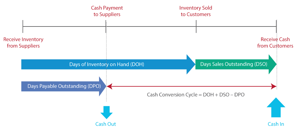
# of days comp takes for inventory investment → cash receipt
= DOH + DSO - DPO |
Operating Cycle | = DOH + DSO |
Working Capital (WC) | Total Working Capital: CA - CL Net Working Capital: CA - CL, excluding cash / MS / ST debt |
Cash Flow from Operations (CFO) | = Cash received from customers + Int and div received on investments
- Cash paid to employees / suppliers - Taxes paid to gov - Int paid to lenders = NI + NCC - WCInv * Does not account for capital investments that issuers make to improve operations |
Free Cash Flow (FCF): | = CFO - Investments in LT assets = Excess of operating cash flow over capital expenditures |
FCF to Firm (FCFF) | = NI + NCC + Int(1 – Tax rate) – FCInv – WCInv = CFO + Int(1 – Tax rate) – FCInv = CF avail to D&E investors after all op expense (ie. income tax) are paid, investments in WC and Fixed Capital made NCC = Non-Cash Charge (Amort, Dep) FCInv = Capital expenditures (ie. equipment) Int(1 – Tax rate) = after-tax interest payments CFO = NI + NCC - WCInv Above calculates Int Paid in CFO. If Int Paid is CFF (Only IFRS), delete Int(1 – Tax rate) If Int Paid is CFI (Only IFRS), add to CFO above If Div Paid is CFO (Only IFRS), add to CFO above
|
FCF to Equity (FCFE) | = CFO + Net Borrowing – FCInv = CF avail to Common Stockholders after op expense & borrowing cost (principal, int) are paid, investments in WC and FC made |
IFRS VS USGAAP |
| IFRS (IASB) | US GAAP (FASB) |
Based on | Principles | Rules |
Development Cost | Capitalized if conditions met | Expense |
IS |
Inventory Valuation | FIFO, Weighted av acceptable | FIFO, LIFO, Weighted av acceptable |
Inventory Measurement | Lower (Cost OR NRV) * NRV Assessment done by item / groups of similar items, asses every period |
| Exception: LIFO / Retail Inventory Methods: Lower (Cost OR Market), where |
Writedown Inventory < Carrying Amount (BS) | Writedown Inventory to NRV loss recorded as expense (IS) for Cost of Sale | (For LIFO method) Writedown Inventory to NRV or MV loss recorded as expense (IS) for COGS |
Inventory Writedown Results | - : Profit, Carrying amount of inventory (BS), Profitability / Liquidity / Solvency ratios +: Profitability ratios (inv / total asset turnover as asset reduces) * CFO not affected by non-cash write-down * Exception: writeup happens in y1, and y2 is reversed |
Inventory Writedown Reversal | Reversal limited to original write-down, recognized as reduction in Cost of Sales (Reduction in Inventory recognized as expense) * (Difference between cost and NRVper kg) × (Inventory) | X |
Inventory Exceptions | Agriculture, forest products, minerals / products, commodity broker-traders: Measured in NRV, or quoted market price if an active market exists. Changes recognized as Profit / Loss in period of change |
Inventory Disclosure | Accounting policy to measure inventory [Cost formula (inventory valuation method) Total carrying amount of inventories / in classification (merchandise, raw material..) Carrying amount of inventories carried at Fair Value - Cost to Sell Inventory recognized as expense (Cost of Sales) Write-down of inventories recognized as expense Reversals of any write-down recognized as reduction in Cost of Sales Circumstances leading to reversal Carrying amount of inventories pledged as security for liab
| All same except 6,7,
+ Disclosure of LIFO liquidations’ (1) significant estimates applicable to inventories (2) any material amount of income |
Non-recurring Items = Unusual / Infrequent | IS: In Continuing Operations but separately below the effect on a net basis, including per share basis
BS: related A&L related as Held for Sale |
BS |
LLA Impairment, PPE Impairment | Impaired if Carrying Amount > Recoverable amount * Recoverable amount = Max (Fair Value - Cost to Sell - Value in Use) * Value in use = PV of expected future CF * Impairment loss (IS) = Carrying amount - Recoverable amount | Unrecoverable if Carrying amount > Undiscounted Expected CF * If unrecoverable, Asset written down to Fair Value * Impairment loss (IS) = Fair Value - Carrying amount |
LLA Reversal | Held for Use / Sale: Yes reversal if Recoverable amount increases (Only Impairment Loss, but no revaluation of Recoverable Amount if Recoverable amount > previous carrying amount) | Asset Held for Use: no reverse Asset Held for Sale: yes reverse if Fair Value increases |
Intangible Asset | Cost Model or Revaluation Model (if active market for intangible asset exists) | Cost Model |
Intangibles Disclosure | * Finite: Useful life (Amort rate), Amort method, Gross carrying amount, Accum amort at beg / end of period, Reconciliation of carrying amount at beg / end period * Indefinite: Carrying amount of asset, Why indefinite, Restriction on title and pledges as security, Contractual agreements to acquire intangible assets * Revaluation mode: Date of revelation, How fair value obtained, Carrying amount under cost model, Revelation surplus | Gross carrying amount, Accum amort in total / major class, Aggregate amort expense, Estimated amort expense for next 5 fiscal yrs |
Imp Disclosure | Imp loss / reversal recognized, Where it is in FS, Assets affected by imp / reversal | Description of imp asset, Reason for imp, Method to determine fair value, Amount of imp loss, Where they are recognized in FS |
CFS |
Div / int classification | Flexible Int / div received: CFO / CFI Int / div paid: CFO / CFF | Less flexible Int / div received: CFO Int paid: CFO Div paid: CFF |
Bank overdrafts | Cash equivalents | Financing |
Taxes paid | CFO with portion allocatable to CFI or CFF | CFO |
Format of Statement | In/direct, direct encouraged | In/direct, direct encouraged, reconciliation of net income to CFO must be provided |
